Week 3.5 - Deriving 4th order approximation of a 2nd order derivative using Taylor Table method

Aim : To derive the following 4th order approximations of the second-order derivative using

1. Central difference

2. Skewed right-sided difference

3. Skewed left-sided difference

Central Difference Scheme

For Central difference scheme, Order of Accuracy(P) = N (No of orders in the stencil) - Q+1 ( Order of derivative for symmetric/central scheme)

where P = 4 ; Q = 2 which gives N = P + Q -1 = 4+2-1 = 5

As central difference scheme is symmetric on both sides, so the nodes selected are (i -2) , (i -1), (i), (i +1), (i+2)

Taylor Table For Central Difference Scheme

`(∂^2 f)/(∂x^2)` = a f(i-2) + b f(i-1) + c f (i) + d f(i+1) + e f(i+2)

Stencils	f(i)	f'(i)Δx	f''(i)Δx^2	f'''(i)Δx^3	f''''(i)Δx^4
af(i-2)	a	-2a	4a/2	-8a/6	16a/24
bf(i-1)	b	-b	b/2	-b/6	b/24
c f(i)	c	0	0	0	0
df(i+1)	d	d	d/2	d/6	d/24
ef(i+2)	e	2e	4e/2	8e/6	16e/24
Sum of all terms	0	0	1	0	0

a+b+c+d+e=0 ..(1)

-2a-b+0+d+2e=0....(2)

2a+0.5b+0+0.5d+2e=1...(3)

-8a/6-b/6+0+d/6+8e/6=0....(4)

16a/24+b/24+0+d/24+16e/24=0....(5)

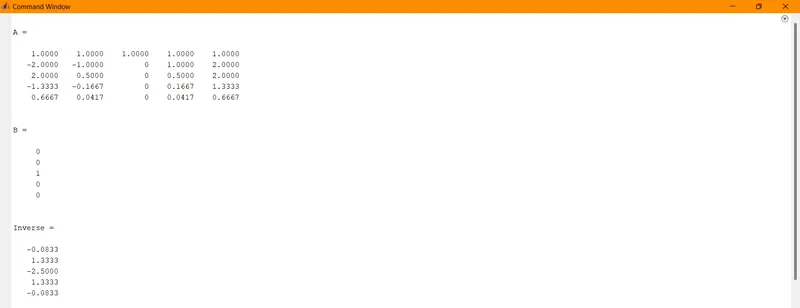
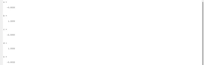
where a = -0.0833 , b = 1.3333 , c = -2.5000 , d = 1.3333 , e = -0.0833

Skewed Right-Sided Difference Scheme

For Skewed Right Sided Difference Scheme Order of Accuracy(P) = N (No of orders in the stencil) - Q( Order of derivative for one sided skewed scheme)

where P = 4 ; Q = 2 which gives N = P + Q = 4+2 = 6

`(∂^2 f)/(∂x^2)` = a f(i) + b f(i+1) + c f (i+2)+ d f(i+3) + e f(i+4)+gf(i+5)

Stencils	f(i)	f'(i)Δx	f''(i)Δx^2	f'''(i)Δx^3	f''''(i)Δx^4	f'''''(i)Δx^5
af(i)	a	0	0	0	0	0
bf(i+1)	b	b	b/2	b/6	b/24	b/120
c f(i+2)	c	2c	4c/2	8c/6	16c/24	32c/120
d f(i+3)	d	3d	9d/2	27d/6	81d/24	243d/120
e f(i+4)	e	4e	16e/2	64e/6	256e/24	1024e/120
g f(i+5)	g	5g	25g/2	125g/6	625g/24	3125g/120
Sum of all terms	0	0	1	0	0	0

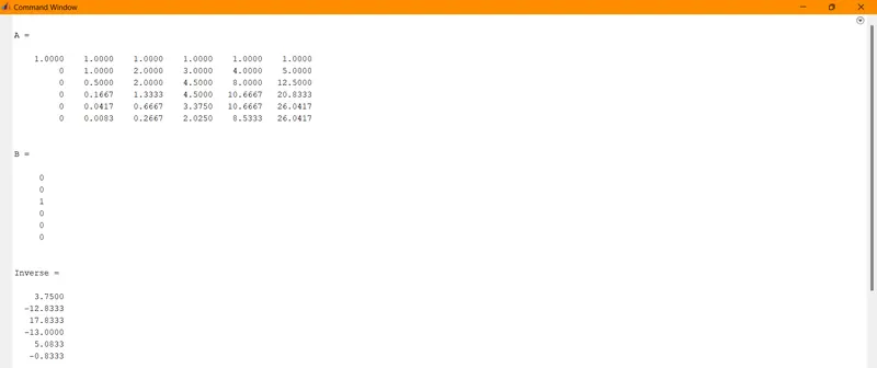
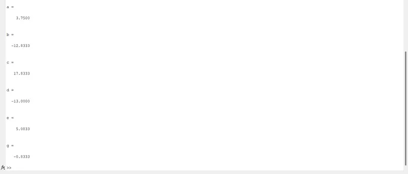
where

a = 3.7500 , b = -12.8333, c = 17.8333, d =-13.0000, e = 5.0833, g = -0.8333

Skewed Left-Sided Difference Scheme

For Skewed Left Sided Difference Scheme Order of Accuracy(P) = N (No of orders in the stencil) - Q( Order of derivative for one sided skewed scheme)

where P = 4 ; Q = 2 which gives N = P + Q = 4+2 = 6

`(∂^2 f)/(∂x^2)` = a f(i) + b f(i-1) + c f (i-2)+ + d f(i-3) + e f(i-4)+gf(i-5)

Stencils	f(i)	f'(i)Δx	f''(i)Δx^2	f'''(i)Δx^3	f''''(i)Δx^4	f'''''(i)Δx^5
af(i)	a	0	0	0	0	0
bf(i-1)	b	-b	b/2	-b/6	b/24	-b/120
c f(i-2)	c	-2c	4c/2	-8c/6	16c/24	-32c/120
d f(i-3)	d	-3d	9d/2	-27d/6	81d/24	-243d/120
e f(i-4)	e	-4e	16e/2	-64e/6	256e/24	-1024e/120
g f(i-5)	g	-5g	25g/2	-125g/6	625g/24	-3125g/120
Sum of all terms	0	0	1	0	0	0

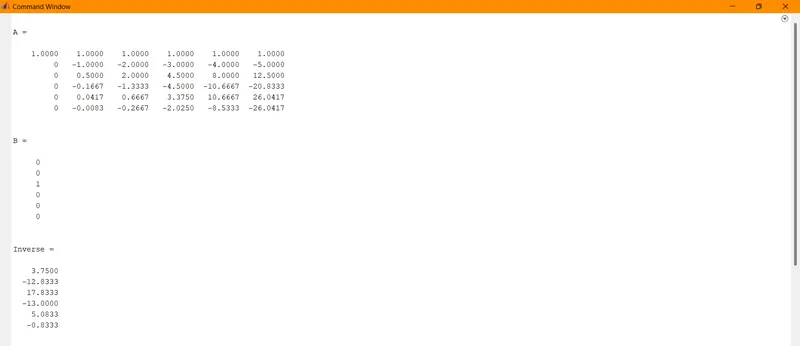
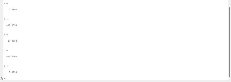
where

a = 3.7500 , b = -12.8333, c = 17.8333, d =-13.0000, e = 5.0833, g = -0.8333

Function Code For Central Difference Scheme

function error = central_difference(analytical_derivative,x,dx)
%% Matrix Equation AX=B
A = [1 1 1 1 1;-2 -1 0 1 2;4/2 1/2 0 1/2 4/2; -8/6 -1/6 0 1/6 8/6;16/24 1/24 0 1/24 16/24]
B = [0;0;1;0;0]
%% Inverse Of the Matrix
X = inv(A)*B 
%% Central Difference Scheme
f1=exp(x-2*dx)*cos(x-2*dx);
f2=exp(x-dx)*cos(x-dx);
f3=exp(x)*cos(x);
f4=exp(x+dx)*cos(x+dx);
f5=exp(x+2*dx)*cos(x+2*dx);
central_difference=((X(1)*f1)+(X(2)*f2)+(X(3)*f3)+(X(4)*f4)+(X(5)*f5))/(dx^2);
%% Error Calculation
error=abs(analytical_derivative-central_difference);
end

Function Code For Skewed Right-Sided Difference Scheme

function error = skewed_right_difference(analytical_derivative,x,dx)
%% Matrix Equation CX=D
C = [1 1 1 1 1 1;0 1 2 3 4 5;0 1/2 2 9/2 16/2 25/2;0 1/6 8/6 27/6 64/6 125/6;0 1/24 16/24 81/24 256/24 625/24;0 1/120 32/120 243/120 1024/120 3125/120]
D = [0;0;1;0;0;0]
%% Inverse Of the Matrix
Y = inv(C)*D
%% Skewed Right-Sided Difference Scheme
f1=exp(x)*cos(x);
f2=exp(x+dx)*cos(x+dx);
f3=exp(x+2*dx)*cos(x+2*dx);
f4=exp(x+3*dx)*cos(x+3*dx);
f5=exp(x+4*dx)*cos(x+4*dx);
f6=exp(x+5*dx)*cos(x+5*dx);
skewed_right_difference=((Y(1)*f1)+(Y(2)*f2)+(Y(3)*f3)+(Y(4)*f4)+(Y(5)*f5)+(Y(6)*f6))/(dx^2);
%% Error Calculation
error=abs(analytical_derivative-skewed_right_difference);
end

Function Code For Skewed Left-Sided Difference Scheme

function error = skewed_left_difference(analytical_derivative,x,dx)
%% Matrix Equation EX=F
E = [1 1 1 1 1 1;-5 -4 -3 -2 -1 0;25/2 16/2 9/2 4/2 1/2 0;-125/6 -64/6 -27/6 -8/6 -1/6 0;625/24 256/24 81/24 16/24 1/24 0;-3125/120 -1024/120 -243/120 -32/120 -1/120 0]
F = [0;0;1;0;0;0]
%% Inverse Of the Matrix
Z = inv(E)*F
%% Skewed Left-Sided Difference Scheme
f1=exp(x-5*dx)*cos(x-5*dx);
f2=exp(x-4*dx)*cos(x-4*dx);
f3=exp(x-3*dx)*cos(x-3*dx);
f4=exp(x-2*dx)*cos(x-2*dx);
f5=exp(x-dx)*cos(x-dx);
f6=exp(x)*cos(x);
skewed_left_difference=((Z(1)*f1)+(Z(2)*f2)+(Z(3)*f3)+(Z(4)*f4)+(Z(5)*f5)+(Z(6)*f6))/(dx^2);
%% Error Calculation
error=abs(analytical_derivative-skewed_left_difference);
end

Main Code

clear all;
close all;
clc;
%% Given Inputs
x=pi/3;
dx=linspace(pi/4,pi/400,20);
%% Given Equation
f=exp(x)*cos(x);
%% Analytical_Derivative
analytical_derivative = -2*exp(x)*sin(x);
%% For Loop
for i=1:length(dx)
    central_error(i) = central_difference(analytical_derivative,x,dx(i));
    skewed_right_error(i) = skewed_right_difference(analytical_derivative,x,dx(i));
    skewed_left_error(i) = skewed_left_difference(analytical_derivative,x,dx(i));
end
%% Plotting
figure(1)
loglog(dx,central_error,'color','#941d50',"LineWidth",1);
hold on;
loglog(dx,skewed_right_error,'color','#055E7A',"LineWidth",1);
hold on;
loglog(dx,skewed_left_error,'color','#012710',"linewidth",1);
%% Labelling
xlabel('dx',"FontSize",14,"FontName","Times New Roman");
ylabel('Absolute error',"FontSize",12,"FontName","SansSerif");
title('Consistency of different scheme',"FontSize",9,"FontName","Cambria");
legend('Central Difference','Skewed Right-Sided','Skewed Left-Sided',"FontSize",10,"FontName","Cambria",Location='southeast');
grid on;

Output Plot

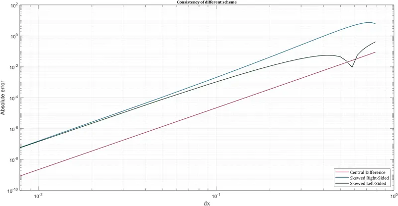
Describe why a skewed scheme is useful? What can a skewed scheme do that a CD scheme cannot?

• Skewed schemes come in handy when we don't have the data from both sides of the nodes. As in the skewed scheme, one side of the data is sufficient to compute the numerical approximation, whereas in the central difference scheme, we need data inputs from both sides of the nodes.
• On the other hand, the central difference scheme gives more efficient outputs than the skewed scheme,but it is not always feasible to go with the Central Difference method due to input data deficiency.