Week 3.5 - Deriving 4th order approximation of a 2nd order derivative using Taylor Table method

Aim: To derive the 4th order approximations of the second-order derivative.

1) Central differencing:

First we find the 4th order approximations of the second-order derivative by using Central differencing method of Taylor table method. In this method we take information from both back and front side nodes,

for central differencing the number of stencil nodes are calculated by

The order of accuracy P = Number of nodes in the stencil N - order of derivative Q + 1

hence,

Number of nodes in the stencil N = The order of accuracy P + order of derivative Q - 1

N= 4+2-1

N=5

therefore the equation is,

∂²f/∂x²= a f(i−2) + b f(i−1) + c f(i) + d f(i+1) + e f(i+2)

Taylor table

	f(X)	dx f’(x)	dx2 f’’(x)	dx3 f’’’(x)	dx4 f’’’’(x)	dx5 f’’’’’(x)
a f(i-1)	a	-2a	4a/2	-8a/6	16a/24	-32a/120
b f(i-2)	b	-b	b/2	-b/6	b/24	-b/120
c f(i)	c	0	0	0	0	0
d f(i-1)	d	d	d/2	d/6	d/24	d/120
e f(i-2)	e	2e	4e/2	8e/6	16e/24	32e/120
a f(i-2) +bf(i-1) +cf(i) +df(i+1) + ef(i+2)	0	0	1	0	0	?

Next we arrange above values in matrix form

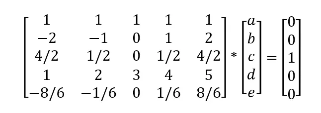
we solving this matrix by using matlab and find the value of a,b,c,d,e as follows

a=-0.0833, b=1.3333, c=-2.5000, d=1.3333, e=-0.0833

2) Skewed right-sided difference:-

Number of nodes in the stencil N = The order of accuracy P + order of derivative Q

N= 4+2

N=6

therefore the equation is,

∂²f/∂x²= a f(i) + b f(i+1) + c f(i+2) + d f(i+3) + e f(i+4) + g f(i+5)

	f(X)	dx f’(x)	dx2 f’’(x)	dx3 f’’’(x)	dx4 f’’’’(x)	dx5 f’’’’’(x)
af(i)	a	0	0	0	0	0
bf(i+1)	b	b	b/2	b/6	b/24	b/120
cf(i+2)	c	2c	4c/2	8c/6	16c/24	32c/120
df(i+3)	d	3d	9d/2	27d/6	81d/24	243d/120
ef(i+4)	e	4e	16e/2	64e/6	256e/24	1024e/120
ff(i+5)	g	5g	25g/2	125g/6	625g/24	3125g/120
af(i) + bf(i+1) + cf(i+2) + df(i+3) + ef(i+4) +g f(i+5)	0	0	1	0	0	0

Next we arrange above values in matrix form

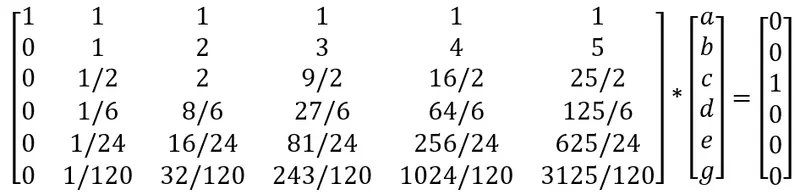
we solving this matrix by using matlab and find the value of a,b,c,d,e as follows

a=3.7500, b=-12.8333 c=17.8333, d=-13.0000, e=5.0833, g=-0.8333

3) Skewed left-sided difference:

Number of nodes in the stencil N = The order of accuracy P + order of derivative Q

N= 4+2

N=6

therefore the equation is,

∂²f/∂x²=a f(i−5) + b f(i−4) + c f(i−3) + d f(i−2) + e f(i−1) + g f(i)

	f(X)	dx f’(x)	dx2 f’’(x)	dx3 f’’’(x)	dx4 f’’’’(x)	dx5 f’’’’’(x)
a f(i-5)	a	-5a	25a/2	-125a/6	625a/24	-3125a/120
b f(i-4)	b	-4b	16b/2	-64b/6	256b/24	-1024b/120
c f(i-3)	c	-3c	9c/2	-27c/6	81c/24	-243c/120
d f(i-2)	d	-2d	4d/2	-8d/6	16d/24	-32d/120
e f(i-1)	e	-e	e/2	-e/6	e/24	-e/120
g f(i)	g	0	0	0	0	0
af(i-5) + bf(i-4) + cf(i-3) + df(i-2) + ef(i-1) +gf(i)	0	0	1	0	0	0

Next we arrange above values in matrix form

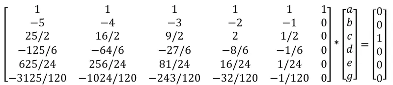
we solving this matrix by using matlab and find the value of a,b,c,d,e as follows

a=-0.8333, b=5.0833 c=13.0000, d=77.8333, e=-12.8333, g=3.7500

matlab code:

Defining the function.

1) Central difference

function Error_central_differencing = fourth_order_central_differencing(x,dx)

% analytic function = exp(x)*cos(x)

% analytic derivative
%f''(x) = -2*exp(x)*sin(x)

analytical_derivative = -2*exp(x)*sin(x);

%numerical derivative

%central differencing
central_differencing = (((-0.0833)*((exp(x-(2*dx)))*(cos(x-(2*dx)))))+((1.3333)*((exp(x-dx))*(cos(x-dx))))-((2.5000)*((exp(x))*(cos(x))))+((1.3333)*((exp(x+dx))*(cos(x+dx))))-((0.0833)*((exp(x+(2*dx)))*(cos(x+(2*dx))))))/(dx^2);

%error
Error_central_differencing = abs(central_differencing- analytical_derivative);
end

2)Skewed right-sided difference

function Error_right_sided_skew = fourth_order_right_sided_skew(x,dx)

% analytic function = exp(x)*cos(x)

% analytic derivative
%f''(x) = -2*exp(x)*sin(x)

analytical_derivative = -2*exp(x)*sin(x);

%numerical derivative

%central differencing
right_sided_skew = (((3.7500)*((exp(x))*(cos(x))))-((12.8333)*((exp(x+dx))*(cos(x+dx))))+((17.8333)*((exp(x+(2*dx)))*(cos(x+(2*dx)))))-((13.0000)*((exp(x+(3*dx)))*(cos(x+(3*dx)))))+((5.0833)*((exp(x+(4*dx)))*(cos(x+(4*dx)))))-((0.8333)*((exp(x+(5*dx)))*(cos(x+(5*dx))))))/(dx^2);

%error
Error_right_sided_skew = abs(right_sided_skew- analytical_derivative);
end

3) Skewed left-sided difference

function Error_left_sided_skew = fourth_order_left_sided_skew(x,dx)

% analytic function = exp(x)*cos(x)

% analytic derivative
%f''(x) = -2*exp(x)*sin(x)

analytical_derivative = -2*exp(x)*sin(x);

%numerical derivative

%central differencing
left_sided_skew = (((-0.8333)*((exp(x-(5*dx)))*(cos(x-(5*dx)))))+((5.0833)*((exp(x-(4*dx)))*(cos(x-(4*dx)))))-((13.0000)*((exp(x-(3*dx)))*(cos(x-(3*dx)))))+((17.8333)*((exp(x-(2*dx)))*(cos(x-(2*dx)))))-((12.8333)*((exp(x-dx))*(cos(x-dx))))+((3.7500)*((exp(x))*(cos(x)))))/(dx^2);

%error
Error_left_sided_skew = abs(left_sided_skew- analytical_derivative);
end

Main Programm

clear all
close all
clc

%value of x
x= pi/3;

%range of dx
dx= linspace(pi/4,pi/4000,20);

%for loop
for i=1:length(dx)
    
    central_differencing(i) = fourth_order_central_differencing(x,dx(i));
    
    right_sided_skew(i) = fourth_order_right_sided_skew(x,dx(i));
    
    left_sided_skew(i) = fourth_order_left_sided_skew(x,dx(i));
    
end

%plotting
figure(1)
loglog(dx,central_differencing,'r','linewidth',3)
hold on
loglog(dx,right_sided_skew,'g','linewidth',3)
hold on
loglog(dx,left_sided_skew,'b','linewidth',3)
xlabel('range of dx')
ylabel('truncation error')
title('range of dx vs error')
legend('central differencing','skewed right sided difference','skewed left sided difference','location','northwest')

RESULT

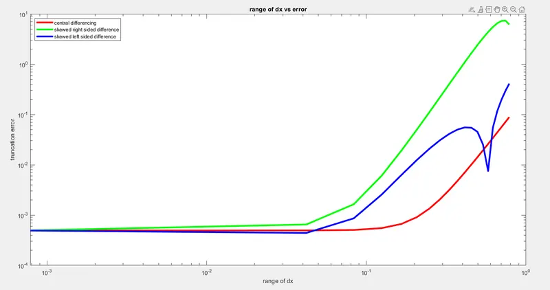
Conclusion:

From this challenge we study the 1)central defferencing, 2) Skewed right-sided difference & 3) Skewed left-sided difference scheme for calculating the 4th order approximations of the second-order derivative. and we found that central difference scheme gives the most accurate results as compare to another two scheme.