Week 3.5 - Deriving 4th order approximation of a 2nd order derivative using Taylor Table method

Central differencing Scheme

Number of nodes

The order of accuracy P = Number of nodes in the stencil N - order of derivative Q + 1

N = P + Q - 1

= 2 + 4 - 1

= 5

Derivation

To derive a fourth order approximation for the second order derivative

expanding all the terms in the above equation using taylor series expansion and are represented in the form of table using taylor table method

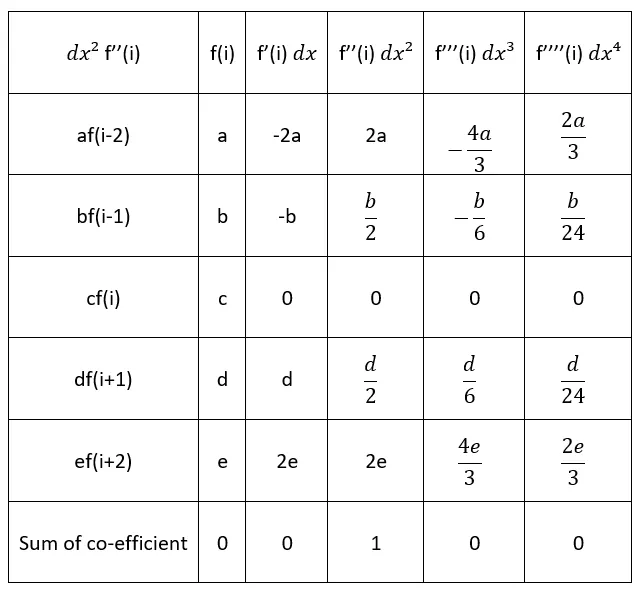
the linear equation obtained from the above table are solved using matrix inversion method

A.X = B

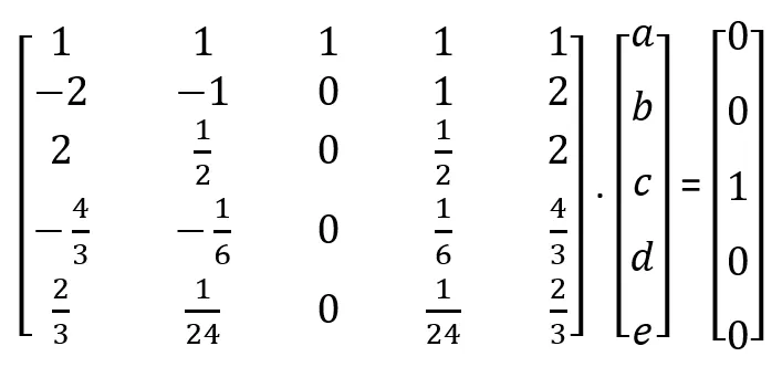
X = inverse(A)*B

we get the co-efficients as,

a = -0.0833, b = 1.3333, c = -2.5000, d = 1.3333 and e = -0.0833

substituting these coefficient we get,

Skewed right-sided difference scheme

Number of nodes

The order of accuracy P = Number of nodes in the stencil N - order of derivative Q

N = P + Q

= 2 + 4

= 6

Derivation

To derive a fourth order approximation for the second order derivative

expanding all the terms in the above equation using taylor series expansion and are represented in the form of table using taylor table method

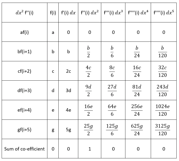
the linear equation obtained from the above table are solved using matrix inversion method

A.X = B

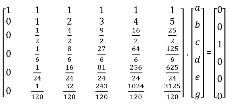
X = inverse(A)*B

we get the co-efficients as,

a = 3.7500, b = -12.8333, c = 2.5000, d = -13.000, e = 5.0833 and g = -0.8333

substituting these coefficient we get,

Skewed left-sided difference scheme

Number of nodes

The order of accuracy P = Number of nodes in the stencil N - order of derivative Q

N = P + Q

= 2 + 4

= 6

Derivation

To derive a fourth order approximation for the second order derivative

expanding all the terms in the above equation using taylor series expansion and are represented in the form of table using taylor table method

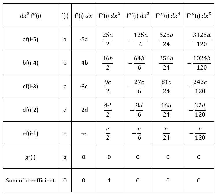
the linear equation obtained from the above table are solved using matrix inversion method

A.X = B

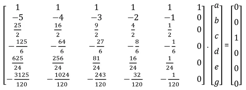
X = inverse(A)*B

we get the co-efficients as,

a = -0.8333, b = 5.0833, c = -13.0000, d = 17.8333, e = -12.8333 and g = 3.7500

substituting these coefficient we get,

Main program

clear all
close all
clc

% value of x
x= pi/3;

% range of dx
dx= linspace(pi/40,pi/4000,20);


for i=1:length(dx)
    
    central_differencing(i) = fourth_order_central_differencing(x,dx(i));
    
    right_sided_skew(i) = fourth_order_right_sided_skew(x,dx(i));
    
    left_sided_skew(i) = fourth_order_left_sided_skew(x,dx(i));
    
end

% plotting
figure(1)
loglog(dx,central_differencing,'color','g')
hold on
loglog(dx,right_sided_skew,'color','r')
hold on
loglog(dx,left_sided_skew,'color','b')
xlabel('range of dx')
ylabel('truncation error')
title('range of dx vs error')
legend('central differencing','right sided skew','left sided skew')

Function code for central differencing

function Error_central_differencing = fourth_order_central_differencing(x,dx)

% analytic function = exp(x)*cos(x)

% analytic derivative
analytical_derivative = -2*exp(x)*sin(x);

% central differencing
central_differencing = (((-0.0833)*((exp(x-(2*dx)))*(cos(x-(2*dx)))))+((1.3333)*((exp(x-dx))*(cos(x-dx))))-((2.5000)*((exp(x))*(cos(x))))+((1.3333)*((exp(x+dx))*(cos(x+dx))))-((0.0833)*((exp(x+(2*dx)))*(cos(x+(2*dx))))))/(dx^2);

% error
Error_central_differencing = abs(central_differencing- analytical_derivative);
end

Function code for skewed-right sided difference

function Error_right_sided_skew = fourth_order_right_sided_skew(x,dx)

% analytic function = exp(x)*cos(x)

% analytic derivative
analytical_derivative = -2*exp(x)*sin(x);

% central differencing
right_sided_skew = (((3.7500)*((exp(x))*(cos(x))))-((12.8333)*((exp(x+dx))*(cos(x+dx))))+((17.8333)*((exp(x+(2*dx)))*(cos(x+(2*dx)))))-((13.0000)*((exp(x+(3*dx)))*(cos(x+(3*dx)))))+((5.0833)*((exp(x+(4*dx)))*(cos(x+(4*dx)))))-((0.8333)*((exp(x+(5*dx)))*(cos(x+(5*dx))))))/(dx^2);

% error
Error_right_sided_skew = abs(right_sided_skew- analytical_derivative);
end

Function code for skewed-left sided difference

function Error_left_sided_skew = fourth_order_left_sided_skew(x,dx)

% analytic function = exp(x)*cos(x)

% analytic derivative
analytical_derivative = -2*exp(x)*sin(x);

% central differencing
left_sided_skew = (((-0.8333)*((exp(x-(5*dx)))*(cos(x-(5*dx)))))+((5.0833)*((exp(x-(4*dx)))*(cos(x-(4*dx)))))-((13.0000)*((exp(x-(3*dx)))*(cos(x-(3*dx)))))+((17.8333)*((exp(x-(2*dx)))*(cos(x-(2*dx)))))-((12.8333)*((exp(x-dx))*(cos(x-dx))))+((3.7500)*((exp(x))*(cos(x)))))/(dx^2);

% error
Error_left_sided_skew = abs(left_sided_skew- analytical_derivative);
end

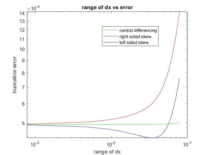
Results

Conclusion

It is observed that central differencing scheme has less error compared with other two schemes such as right sided skew and left sided skew.

Main difference is that one sided/skewed schemes requires data from one end and central differencing scheme requires data from both end.

In order to calculate error at boundary it is difficult to use central differencing scheme in such case we can apply skewed schemes.