Week 3.5 - Deriving 4th order approximation of a 2nd order derivative using Taylor Table method

here u can find the code which is used for solving and finding errors for different skewed approximation system of equations...but i have used a single code without calling it in different function as u have not mentioned a way on what basis it should be followed, so I have followed this simple way

clear all;close all;clc;

set(groot,'DefaultLineLineWidth',3);
set(0,'DefaultAxesFontSize',20);
set(0,'DefaultAxesGridAlpha',0.6);
set(0,'DefaultAxesMinorGridAlpha',0.3);
set(0,'DefaultAxesXminorTick','On');
set(0,'DefaultAxesYminorTick','On');

%% SECTION -1 ---> Assigning Matrix For Finding desired Variables a,b,c,....

%  Matrix considered in the form of [A][X]=[B]
% where A is the matrix of taylor series term
% where B is the matrix of RHS of approximation equation
% where X is the matrix of unknown variable in the LHS of equation

% Right Side Skewed Matrix
RS=[1 1 1 1 1 1; 0 1 2 3 4 5; 0 1/2 2 9/2 8 25/2; 
    0 1/6 4/3 27/6 64/6 125/6; 0 1/24 16/24 81/24 256/24 625/24; 0 1/120 32/120 243/120 1024/120 3125/120];

% Left Side Skewed Matrix
LS=[1 1 1 1 1 1; 0 -1 -2 -3 -4 -5; 0 1/2 2 9/2 8 25/2; 
    0 -1/6 -4/3 -27/6 -64/6 -125/6; 0 1/24 16/24 81/24 256/24 625/24; 0 -1/120 -32/120 -243/120 -1024/120 -3125/120];

% Central Skewed  Matrix
CS=[1 1 1 1 1; -2 -1 0  1 2; 2 1/2 0 1/2 2; -4/3 -1/6 0  1/6 4/3; 2/3 1/24 0 1/24 2/3];

% RHS matrix for Right and left Skewed approximation
B=[0;0;1;0;0;0];

% RHS matrix for Central Skewed approximation
% Here in central skewed approx
%we have No. of nodes= derivative order(P) + approx order(Q)-1
% here P=2; Q=4; hence no.of nodes=5;
B1=[0;0;1;0;0];

%Calculating Unknown Variables for Right_skewed_apprx using matrix
%inversion X=inv(A)*B;

% U can find the corresponding unknown variables in workspace

X1=RS\B;

%Calculating Unknown Variables for Left_skewed_apprx
X2=LS\B;

%Calculating Unknown Variables for Central_skewed_apprx
X3=CS\B1;

% Assigning inputs
x=pi/3;
dx=linspace(pi/4,pi/4000,40); % assigning grid discritizing

% Actual Given Funnction
Func=exp(x)*cos(x);

%  Actual Second Order Derivative ---> Analytical Solution
actual_soln=-(2*exp(x)*sin(x));

%% SECTION - 2 --->finding error for diff approx using for system of equation

for i=1:(length(dx))
    
    %Right Skewed Approximation Equation
    Right_skewed_soln(i)=(X1(1)*(exp(x)*cos(x)) + X1(2)*(exp(x+dx(i))*cos(x+dx(i))) + X1(3)*(exp(x+(2*dx(i)))*cos(x+(2*dx(i)))) + X1(4)*(exp(x+(3*dx(i)))*cos(x+(3*dx(i)))) + X1(5)*(exp(x+(4*dx(i)))*cos(x+(4*dx(i)))) + X1(6)*(exp(x+(5*dx(i)))*cos(x+(5*dx(i)))))/(dx(i)^2);
    
    %Left Skewed Approximation Equation
    Left_skewed_soln(i)=(X2(1)*(exp(x)*cos(x)) + X2(2)*(exp(x-dx(i))*cos(x-dx(i))) + X2(3)*(exp(x-(2*dx(i)))*cos(x-(2*dx(i)))) + X2(4)*(exp(x-(3*dx(i)))*cos(x-(3*dx(i)))) + X2(5)*(exp(x-(4*dx(i)))*cos(x-(4*dx(i)))) + X2(6)*(exp(x-(5*dx(i)))*cos(x-(5*dx(i)))))/(dx(i)^2);
    
    %Central Skewed Approximation Equation
    Central_skewed_soln(i)=(X3(1)*(exp(x-(2*dx(i)))*cos(x-(2*dx(i)))) + X3(2)*(exp(x-dx(i))*cos(x-dx(i))) + X3(3)*(exp(x)*cos(x)) + X3(4)*(exp(x+dx(i))*cos(x+dx(i))) + X3(5)*(exp(x+(2*dx(i)))*cos(x+(2*dx(i)))))/(dx(i)*dx(i));
    
    
    % Finding Absolute error for all approximation on comparing with
    % Analytical Solution
    
    Right_skewed_error(i)=abs(Right_skewed_soln(i)-actual_soln);
    
    Left_skewed_error(i)=abs(Left_skewed_soln(i)-actual_soln);
    
    Central_skewed_error(i)=abs(Central_skewed_soln(i)-actual_soln);

end

%%  SECTION - 4 ---> Printing the corresponding variables for Diff Approx. in command window
fprintf('Right Skewed Approx. variable :\n');
fprintf('a= %f b= %f c= %f d= %f e= %f g= %f \n',X1(1),X1(2),X1(3),X1(4),X1(5),X1(6));

fprintf('Left Skewed Approx. variable :\n');
fprintf('a= %f b= %f c= %f d= %f e= %f g= %f \n',X2(1),X2(2),X2(3),X2(4),X2(5),X2(6));

fprintf('Central Skewed Approx. variable :\n');
fprintf('a= %f b= %f c= %f d= %f e= %f \n',X3(1),X3(2),X3(3),X3(4),X3(5));

%% SECTION - 5 --->ploting in log-log scale plot for dx vs error together for all different skewed approximation

figure(1)
loglog(dx,Right_skewed_error);hold on;
loglog(dx,Left_skewed_error);hold on;
loglog(dx,Central_skewed_error);
xlabel('dx');
ylabel('Error');
legend('Right Skewed Error','Left skewed Error','Central skewed Error','location','southeast');
title('Comparing different skewed approximation');
grid on;grid minor;

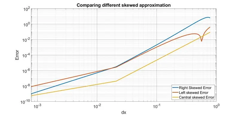
The corresponding output figure is shown here

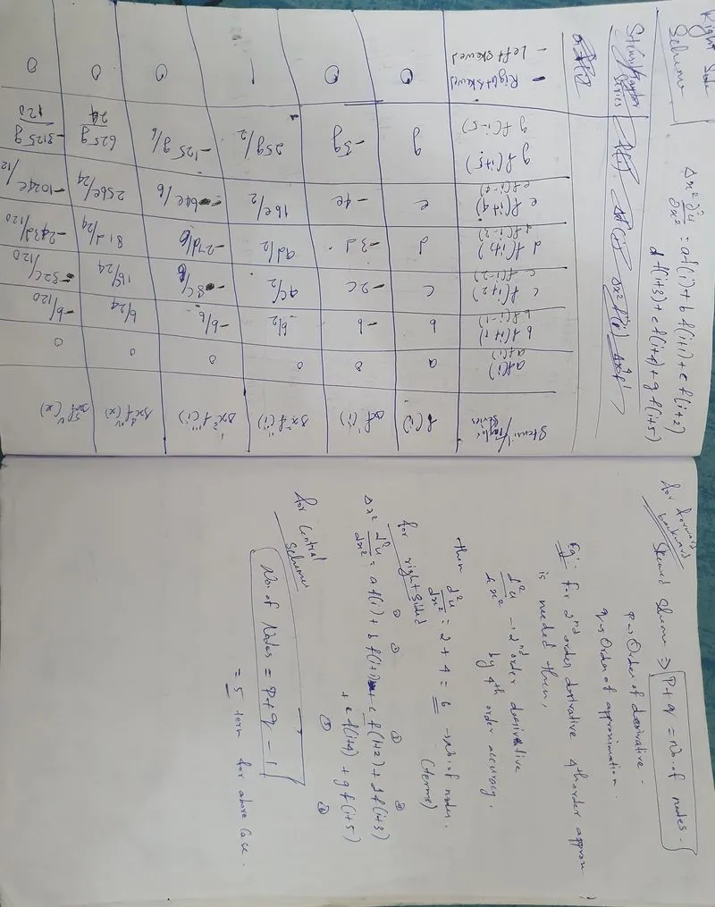
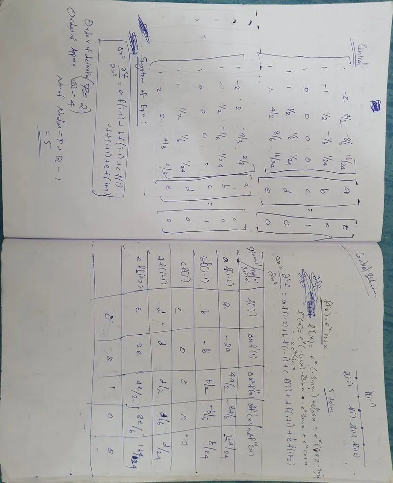
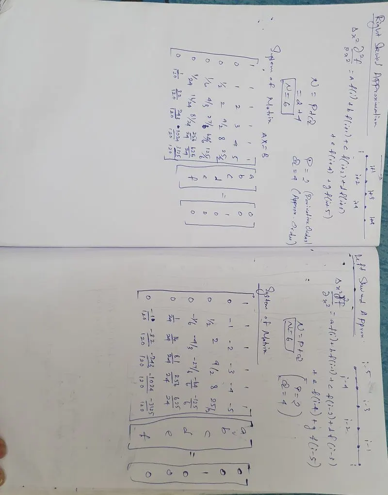
From the above analysis of errors and sysytem equations of different scheme of 4th order approximaton of 2nd order derivative, here I conclude the following observations:

1. Central Scheme has one lesser number of nodes in domain than the both right and left skewed schemes.

2. However Central Scheme is giving less error on comparing with either right/left skewed scheme. The reason behind this inference is that as central scheme is taking the grid points informations on its both side, whereas right/left scheme is taking grid points information on only its either side.

3. Error for all the schemes increases with increase in nodes far apart distance (or) Grid points distance i.e dx

4. However if the grid size is very small i.e <10^-3, the error is not in linear form of increase/decrease, where those error is becoming non-linear solution form of increase/decrease which leads to difficulties to unstabe and finalysing corresponding error. Hence maintaining the precise grid distance is needed to get a appropriate error.

5. Central scheme is showing less error throughtout for a given dx limit than Right/Left scheme.So it is desired to use the Central scheme for more stability and reliable solution.