Week 7 - Simulation of a 1D Supersonic nozzle flow simulation using Macormack Method
Objective:
Simulate the isentropic flow through a quasi 1D subsonic-supersonic nozzle in both the conservation and non-conservation forms of the governing equations and solve them using MacCormack's technique and observe the following results:
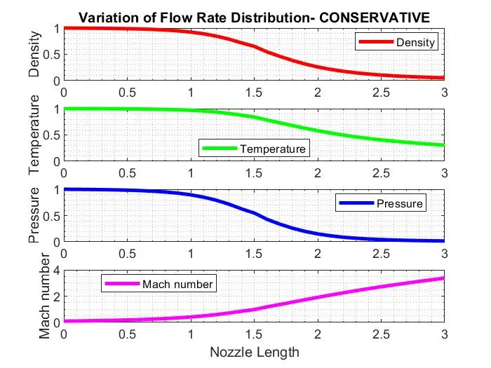
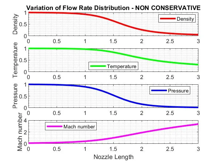
1. Steady-state distribution of primitive variables inside the nozzle
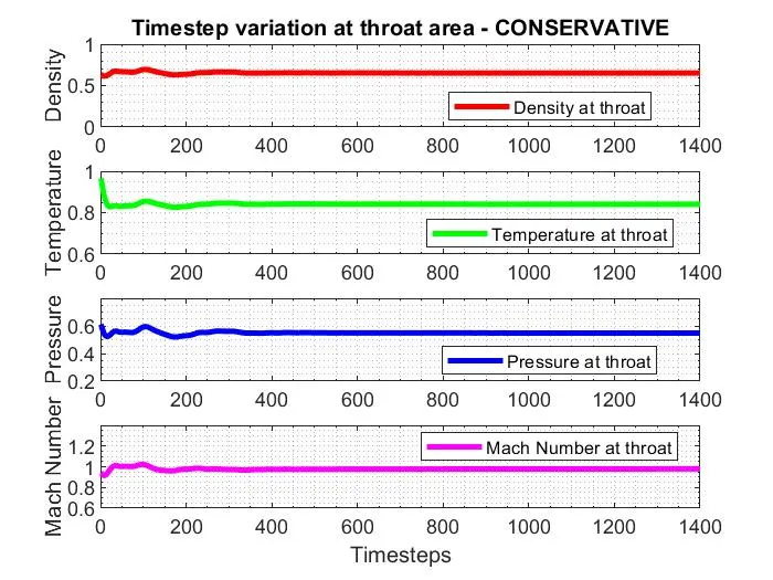
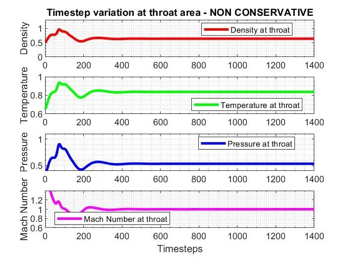
2. Time-wise variation of the primitive variables
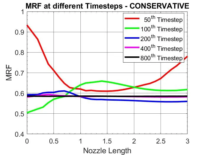
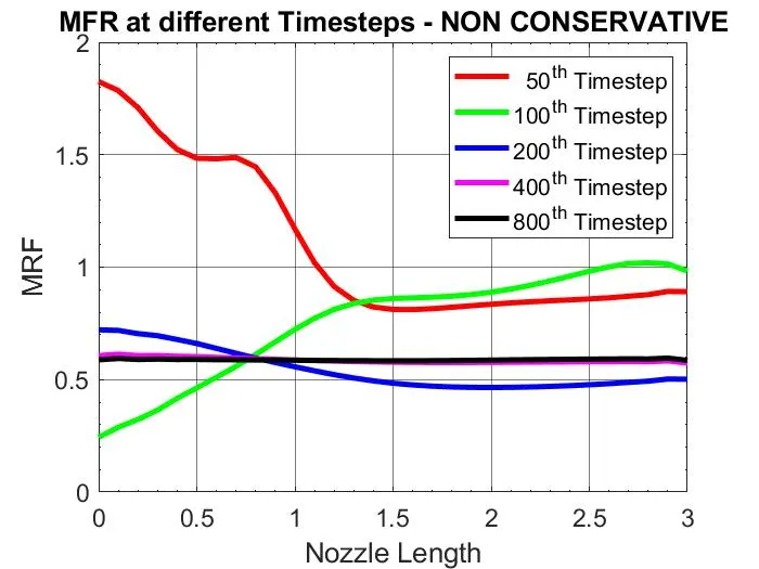
3. Variation of Mass flow rate distribution inside the nozzle at different time steps during the time-marching process
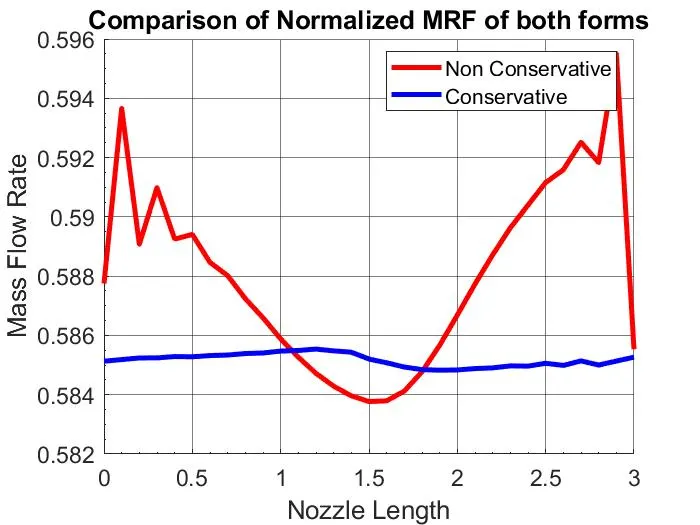
4. Comparison of Normalized mass flow rate distributions of both forms
Matlab Code:
The main code for both conservative and non-conservative forms for solving governing equations using MacCormack's technique is given below:
close all;clear all;clc;

set(groot,'DefaultLineLineWidth',3);
set(0,'DefaultAxesFontSize',14);
set(0,'DefaultAxesGridAlpha',0.6);
set(0,'DefaultAxesMinorGridAlpha',0.3);
set(0,'DefaultAxesXminorTick','On');
set(0,'DefaultAxesYminorTick','On');

n = 31; %Total No. of grid points
gamma = 1.4;
x = linspace(0,3,n);
dx = x(2) - x(1);
nt = 1400; %No. of time step
C = 0.5; %Courant Number

%% Conservative form

[mfr_C, pr_C, mr_C, rho_C, v_C, T_C, rho_throat_C, v_throat_C, T_throat_C, mfr_throat_C, pr_throat_C, mr_throat_C] = cons_function(x, dx, n, gamma, nt, C);
Time_elasped_C = toc;
fprintf('Time Elasped for Conservative form: %0.4f', Time_elasped_C);

%Timestep variation of properties at throat area in Conservative form
figure(2)
�nsity
subplot(4,1,1)
plot(rho_throat_C,'color','r')
ylabel('Density');
legend('Density at throat','location','best');
axis([0 1400 0 1]);
grid minor;
title('Timestep variation at throat area - CONSERVATIVE');
%Temperature
subplot(4,1,2)
plot(T_throat_C,'color','g');
ylabel('Temperature');
legend('Temperature at throat','location','best');
axis([0 1400 0.6 1]);
grid minor;
%Pressure
subplot(4,1,3)
plot(pr_throat_C,'color','b');
ylabel('Pressure');
legend('Pressure at throat','location','best');
axis([0 1400 0.2 0.8]);
grid minor
%Mach Number
subplot(4,1,4)
plot(mr_throat_C,'color','m');
xlabel('Timesteps');
ylabel('Mach Number');
legend('Mach Number at throat','location','best');
axis([0 1400 0.6 1.4]);
grid minor;

%Steady state simulation for primitve values for Non Conservative form
figure(3);
�nsity
subplot(4,1,1)
plot(x,rho_C,'color','r');
ylabel('Density');
legend('Density','location','best');
axis([0 3 0 1]);
grid minor;
title('Variation of Flow Rate Distribution - CONSERVATIVE');
%Temperature
subplot(4,1,2)
plot(x,T_C,'color','g');
ylabel('Temperature');
legend('Temperature','location','best');
axis([0 3 0 1])
grid minor;
%Pressure
subplot(4,1,3)
plot(x,pr_C,'color','b');
ylabel('Pressure')
legend('Pressure','location','best');
axis([0 3 0 1])
grid minor;
%Mach number
subplot(4,1,4)
plot(x,mr_C,'color','m');
xlabel('Nozzle Length');
ylabel('Mach number');
legend('Mach number','location','best');
axis([0 3 0 4])
grid minor;

%% Non-Conservative form

[mfr_NC, pr_NC, mr_NC, rho_NC, v_NC, T_NC, rho_throat_NC, v_throat_NC, T_throat_NC, mfr_throat_NC, pr_throat_NC, mr_throat_NC] = non_cons_function(x, dx, n, gamma, nt, C);
Time_elapsed_NC = toc;
fprintf('Time Elasped for Non Conservative form: %0.4f', Time_elapsed_NC);
hold on;

%Timestep variation of properties at throat area in Non Conservative form
figure(5)
�nsity
subplot(4,1,1)
plot(linspace(1,nt,nt),rho_throat_NC,'color','r');
ylabel('Density');
legend('Density at throat','location','best');
axis([0 1400 0 1.3]);
grid minor;
title('Timestep variation at throat area - NON CONSERVATIVE');
%Temperature
subplot(4,1,2)
plot(linspace(1,nt,nt),T_throat_NC,'color','g');
ylabel('Temperature');
legend('Temperature at throat','location','best');
axis([0 1400 0.6 1]);
grid minor;
%Pressure
subplot(4,1,3)
plot(linspace(1,nt,nt),pr_throat_NC,'color','b');
ylabel('Pressure');
legend('Pressure at throat','location','best');
axis([0 1400 0.4 1.1]);
grid minor
%Mach Number
subplot(4,1,4)
plot(linspace(1,nt,nt),mr_throat_NC,'color','m');
xlabel('Timesteps');
ylabel('Mach Number');
legend('Mach Number at throat','location','best');
axis([0 1400 0.6 1.4]);
grid minor;

%Steady state simulation for primitve values for Non Conservative
figure(6);
�nsity
subplot(4,1,1)
plot(x,rho_NC,'color','r');
ylabel('Density');
legend('Density','location','best');
axis([0 3 0 1]);
grid minor;
title('Variation of Flow Rate Distribution - NON CONSERVATIVE');
%Temperature
subplot(4,1,2)
plot(x,T_NC,'color','g');
ylabel('Temperature');
legend('Temperature','location','best');
axis([0 3 0 1]);
grid minor;
%Pressure
subplot(4,1,3)
plot(x,pr_NC,'color','b');
ylabel('Pressure');
legend('Pressure','location','best');
axis([0 3 0 1]);
grid minor;
%Mach number
subplot(4,1,4)
plot(x,mr_NC,'color','m');
xlabel('Nozzle Length');
ylabel('Mach number');
legend('Mach number','location','best');
axis([0 3 0 4]);
grid minor;

%COMPARISON PLOT of Normalized Mass Flow Rate
figure(7)
hold on
plot(x,mfr_NC,'r');
hold on;
plot(x,mfr_C,'b');
grid on;
legend('Non Conservative','Conservative','location','best');
xlabel('Nozzle Length');
ylabel('Mass Flow Rate');
title('Comparison of Normalized MRF of both forms');
Conservative Form Function:
The call function made for the conservative form is given below:
function [mfr_C, pr_C, mr_C, rho_C, v_C, T_C, rho_throat_C, v_throat_C, T_throat_C, mfr_throat_C, pr_throat_C, mr_throat_C] = cons_function(x, dx, n, gamma, nt, C)
�termining Initial profile of Density and Temperature
for i = 1:n

if (x(i) >= 0 && x(i) <= 0.5)
rho_C(i) = 1;
T_C(i) = 1;
elseif (x(i) >= 0.5 && x(i) <= 1.5)
rho_C(i) = 1 - 0.366*(x(i) - 0.5);
T_C(i) = 1 - 0.167*(x(i) - 0.5);
elseif (x(i) >= 1.5 && x(i) <= 3)
rho_C(i) = 0.634 - 0.3879*(x(i) - 1.5);
T_C(i) = 0.833 - 0.3507*(x(i) - 1.5);
end

end
%Area & Throat profiles
a = 1 + 2.2*(x - 1.5).^2;
throat = find(a==1);
%Initial profile fot Velocity and pr
v_C = 0.59./(rho_C.*a);
pr_C = rho_C.*T_C;
�lculate the Initial Solution Vectors(U)
U1 = rho_C.*a;
U2 = rho_C.*a.*v_C;
U3 = rho_C.*a.*(T_C./(gamma - 1)) + ((gamma/2).*v_C.^2);
%Outer Time Loop
for k =1:nt

%Time-step control
dt = min(C.*dx./(sqrt(T_C) + v_C));

%Saving a copy of Old Values
U1_old = U1;
U2_old = U2;
U3_old = U3;
�lculating the Flux vector(F)
F1 = U2;
F2 = ((U2.^2)./U1) + ((gamma - 1)/gamma)*(U3 - (gamma/2)*((U2.^2)./U1));
F3 = ((gamma*U2.*U3)./U1) - (gamma*(gamma - 1)*((U2.^3)./(2*U1.^2)));


%Predictor Method
for j = 2:n-1

�lculating the Source term(J)
J2(j) = (1/gamma)*rho_C(j)*T_C(j)*((a(j + 1) - a(j))/dx);


%Continuity Equation
dU1_dt_P(j) = -((F1(j + 1) - F1(j))/dx);

%Momentum Equation
dU2_dt_P(j) = -((F2(j + 1) - F2(j))/dx) + J2(j);

%Energy Equation
dU3_dt_P(j) = -((F3(j + 1) - F3(j))/dx);


%Updating New values
U1(j) = U1(j) + dU1_dt_P(j)*dt;
U2(j) = U2(j) + dU2_dt_P(j)*dt;
U3(j) = U3(j) + dU3_dt_P(j)*dt;

end

%Updating Flux vectors
F1 = U2;
F2 = ((U2.^2)./U1) + ((gamma - 1)/gamma)*(U3 - ((gamma*0.5*(U2.^2))./(U1)));
F3 = ((gamma*U2.*U3)./U1) - ((gamma*0.5*(gamma - 1)*(U2.^3))./(U1.^2));

%Corrector Method
for j = 2:n-1

%Updating the Source term(J)
J2(j) = (1/gamma)*rho_C(j)*T_C(j)*((a(j) - a(j - 1))/dx);
%Simplifying the Equation's spatial terms
dU1_dt_C(j) = -((F1(j) - F1(j - 1))/dx);
dU2_dt_C(j) = -((F2(j) - F2(j - 1))/dx) + J2(j);
dU3_dt_C(j) = -((F3(j) - F3(j - 1))/dx);
end
%Compute Average Time derivative
dU1_dt = 0.5*(dU1_dt_P + dU1_dt_C);
dU2_dt = 0.5*(dU2_dt_P + dU2_dt_C);
dU3_dt = 0.5*(dU3_dt_P + dU3_dt_C);
%Final Solution Update
for i = 2:n-1
U1(i) = U1_old(i) + dU1_dt(i)*dt;
U2(i) = U2_old(i) + dU2_dt(i)*dt;
U3(i) = U3_old(i) + dU3_dt(i)*dt;

end


%Applying Boundary Conditions
%At Inlet
U1(1) = rho_C(1)*a(1);
U2(1) = 2*U2(2) - U2(3);

v_C(1) = U2(1)./U1(1);
U3(1) = U1(1)*((T_C(1)/(gamma - 1)) + ((gamma/2)*(v_C(1)).^2));

%At Outlet
U1(n) = 2*U1(n - 1) - U1(n - 2);
U2(n) = 2*U2(n - 1) - U2(n - 2);
U3(n) = 2*U3(n - 1) - U3(n - 2);

%Final Primitive value update
rho_C = U1./a;
v_C = U2./U1;
T_C = (gamma - 1)*((U3./U1 - (gamma/2)*(v_C).^2));

�fining Mass flow rate, pr and Mach number
mfr_C = rho_C.*a.*v_C;
pr_C = rho_C.*T_C;
mr_C = (v_C./sqrt(T_C));

�lculating Variables at throat section
rho_throat_C(k) = rho_C(throat);
T_throat_C(k) = T_C(throat);
v_throat_C(k) = v_C(throat);
mfr_throat_C(k) = mfr_C(throat);
pr_throat_C(k) = pr_C(throat);
mr_throat_C(k) = mr_C(throat);

%Comparison of non-dimensional Mass flow rates at different time steps
figure(1)
if k == 50
plot(x, mfr_C, 'r');
hold on
elseif k == 100
plot(x, mfr_C, 'g');
hold on
elseif k == 200
plot(x, mfr_C, 'b');
hold on
elseif k == 400
plot(x, mfr_C, 'm');
hold on
elseif k == 800
plot(x, mfr_C, 'k');
hold on
end

title('MRF at different Timesteps - CONSERVATIVE');
xlabel('Nozzle Length');
ylabel('MRF');
legend('  50^{th} Timestep','100^{th} Timestep','200^{th} Timestep','400^{th} Timestep','800^{th} Timestep');
axis([0 3 0.4 1]);
grid on

end
end
Non-Conservative Form Function:
The call function made for non-conservative form is given below:
function [mfr_NC, pr_NC, mr_NC, rho_NC, v_NC, T_NC, rho_throat_NC, v_throat_NC, T_throat_NC, mfr_throat_NC, pr_throat_NC, mr_throat_NC] = non_cons_function(x, dx, n, gamma, nt, C)
%Intial boundary conditions
rho_NC = 1 - 0.3146*x;
T_NC = 1 - 0.2341*x;
v_NC = (0.1 + 1.09*x).*T_NC.^0.5;
%Area & Throat profiles
a = 1 + 2.2*(x - 1.5).^2;
throat = find(a==1);


for k = 1:nt

%Time-step control
dt = min(C.*dx./(sqrt(T_NC) + v_NC));

%Saving a copy of Old Values
rho_old = rho_NC;
T_old = T_NC;
v_old = v_NC;

%Predictor Method
for j = 2:n-1

%Simplifying the Equation's spatial terms
dv_dx = (v_NC(j + 1) - v_NC(j))/dx;
drho_dx = (rho_NC(j + 1) - rho_NC(j))/dx;
dT_dx = (T_NC(j + 1) - T_NC(j))/dx;
dlog_a_dx = (log(a(j + 1)) - log(a(j)))/dx;

%Continuity Equation
drho_dt_P(j) = -rho_NC(j)*dv_dx - rho_NC(j)*v_NC(j)*dlog_a_dx - v_NC(j)*drho_dx;

%Momentum Equation
dv_dt_P(j) = -v_NC(j)*dv_dx - (1/gamma)*(dT_dx + (T_NC(j)*drho_dx/rho_NC(j)));

%Energy Equation
dT_dt_P(j) = -v_NC(j)*dT_dx - (gamma - 1)*T_NC(j)*(dv_dx + v_NC(j)*dlog_a_dx);


%Solution Update
rho_NC(j) = rho_NC(j) + drho_dt_P(j)*dt;
v_NC(j) = v_NC(j) + dv_dt_P(j)*dt;
T_NC(j) = T_NC(j) + dT_dt_P(j)*dt;

end


%Corrector Method
for j = 2:n-1

%Simplifying the Equation's spatial terms
dv_dx = (v_NC(j) - v_NC(j - 1))/dx;
drho_dx = (rho_NC(j) - rho_NC(j - 1))/dx;
dT_dx = (T_NC(j) - T_NC(j - 1))/dx;
dlog_a_dx = (log(a(j)) - log(a(j - 1)))/dx;

%Continuity Equation
drho_dt_C(j) = - rho_NC(j)*dv_dx - rho_NC(j)*v_NC(j)*dlog_a_dx - v_NC(j)*drho_dx;

%Momentum Equation
dv_dt_C(j) = - v_NC(j)*dv_dx - (1/gamma)*(dT_dx + (T_NC(j)*drho_dx/rho_NC(j)));

%Energy Equation
dT_dt_C(j) = - v_NC(j)*dT_dx - (gamma - 1)*T_NC(j)*(dv_dx + v_NC(j)*dlog_a_dx);

end

%Compute Average Time derivative
drho_dt = 0.5.*(drho_dt_P + drho_dt_C);
dv_dt = 0.5.*(dv_dt_P + dv_dt_C);
dT_dt = 0.5.*(dT_dt_P + dT_dt_C);

%Final Solution Update
for i = 2:n-1
rho_NC(i) = rho_old(i) + drho_dt(i)*dt;
v_NC(i) = v_old(i) + dv_dt(i)*dt;
T_NC(i) = T_old(i) + dT_dt(i)*dt;

end

%Applying Boundary Conditions
%At Inlet
rho_NC(1) = 1;
v_NC(1) = 2*v_NC(2) - v_NC(3);
T_NC(1) = 1;

%At Outlet
rho_NC(n) = 2*rho_NC(n-1) - rho_NC(n - 2);
v_NC(n) = 2*v_NC(n - 1) - v_NC(n - 2);
T_NC(n) = 2*T_NC(n - 1) - T_NC(n - 2);


�fining Mass flow rate, pr and Mach number
mfr_NC = rho_NC.*a.*v_NC;
pr_NC = rho_NC.*T_NC;
mr_NC = (v_NC./sqrt(T_NC));

�lculating Variables at throat section
rho_throat_NC(k) = rho_NC(throat);
T_throat_NC(k) = T_NC(throat);
v_throat_NC(k) = v_NC(throat);
mfr_throat_NC(k) = mfr_NC(throat);
pr_throat_NC(k) = pr_NC(throat);
mr_throat_NC(k) = mr_NC(throat);


%PLOTTING
%Comparison of non-dimensional Mass flow rates at different time steps
figure(4);
if k == 50
plot(x, mfr_NC, 'r');
hold on
elseif k == 100
plot(x, mfr_NC, 'g');
hold on
elseif k == 200
plot(x, mfr_NC, 'b');
hold on
elseif k == 400
plot(x, mfr_NC, 'm');
hold on
elseif k == 800
plot(x, mfr_NC, 'k');
hold on
end

title('MFR at different Timesteps - NON CONSERVATIVE');
xlabel('Nozzle Length');
ylabel('MRF');
legend('  50^{th} Timestep','100^{th} Timestep','200^{th} Timestep','400^{th} Timestep','800^{th} Timestep');
axis([0 3 0 2]);
grid on

end
endResults:
The output plots from the given code has been enclosed below:
Conclusion:
From the simulation carried out using MacCormack's Technique of solving the governing equations in both conservative and non-conservative forms, we observed the following:
- Density, Temperature, and Pressure parameters decrease along the nozzle length as expected which is similar for both conservative and non-conservative forms whereas the Mach no increases
- As the number of time steps increases, the mass flow rate along the length becomes stable and uniform.
- The Mass Flow Rate is uniform for the conservative form than the Non-conservative form because the mass is conserved in the conservative form which is the expected output whereas the mass flow rate changes throughout the nozzle length for the non-conservative form (minimum at the throat).