Week 3.5 - Deriving 4th order approximation of a 2nd order derivative using Taylor Table method

AIM:

To derive the fourth order approximations of a second order derivative using central differencing scheme, skewed right sided difference and skewed left sided difference with the help of taylor table method and to compare the analytical derivative with obtained values for the given function.

SCHEME DERIVATIONS:

CENTRAL DIFFERENCING SCHEME:

NO OF NODES:

The number of nodes = p+q-1

Where, p is order of derivative.

q is order of approximations.

The no of nodes = 2+4-1 =>5.

DERIVATION:

To derive a fourth order approximation for the second order derivative,we start with these approximation,

`frac(partial^2 y)(partial^2 x) = a*f(i-2)+b*f(i-1)+c*f(i)+d.f(i+1)+e*f(i+2)` --------------(1)

taylor series derivation for the above terms,

`a*f(i-2)=a*f(i)-frac(2*a*f'(i)*dx)(1!)+frac(4*a*f''(i)*dx^2)(2!)-frac(8*a*f'''(i)*dx^3)(3!)+frac(16*a*f^(iv)(i)*dx^4)(4!)`

Simillarly expand all the terms in the equation (1) and are represented in the form of table using taylor table method.

`dx^2*f''(i)`	`f(i)`	`f'(i)*dx`	`f''(i)*dx^2`	`f'''(i)dx^3`	`f^(iv)(i)dx^4`	`f^(v)(i)dx^5`
af(i-2)	a	-2a	4a/2	-8a/6	16a/24	-32a/120
bf(i-1)	b	-b	b/2	-b/6	b/24	-b/120
cf(i)	c	0	0	0	0	0
df(i+1)	d	d	d/2	d/6	d/24	d/120
ef(i+2)	e	2e	4e/2	8e/6	16e/24	32e/120

Sum of Coefficient

0

0

1

0

0

the linear equation obtained from the above table are solved using matrix inversion method,

A.X = B

A=`[[1,1,1,1,1],[-2,-1,0,1,2],[4/2,1/2,0,1/2,4/2],[-8/6,-1/6,0,1/6,8/6],[16/24,1/24,0,1/24,16/24]]`;

X=`[[a],[b],[c],[d],[e]]`;

B= `[[0],[0],[1],[0],[0]]`;

X=A\B;

We get X as shown below

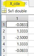
Substitute the values of X_cda matrix in equation (1) and find the second derivative using central difference method.

Here, we observed that a=-0.0833;b=1.3333;c=-2.5;d=1.3333;e=-0.8333;

a=e;b=d;

Substitute in the table for `f^(v)(i)dx^5`and we find that their sum of coefficient = 0;

After that, the term is `f^(vi)(i)dx^6`.

Divide `f^(vi)(i)dx^6`/ `dx^2`, we get the coefficient in the order of `dx^4`. We are neglecting that terms, so we can say that our approximation is fourth order accurate.

SKEWED RIGHT HAND DIFFERENCE SCHEME:

NO OF NODES:

The number of nodes = p+q

Where, p is order of derivative.

q is order of approximations.

The no of nodes = 2+4 =>6.

DERIVATION:

To derive a fourth order approximation for the second order derivative,we start with these approximation,

`frac(partial^2 y)(partial^2 x) = a*f(i)+b*f(i+1)+c*f(i+2)+d.f(i+3)+e*f(i+4)+g*f(i+5)` --------------(2)

expand all the terms in the equation (2) using taylor series expansion and are represented in the form of table using taylor table method.

`dx^2*f''(i)`	`f(i)`	`f'(i)*dx`	`f''(i)*dx^2`	`f'''(i)dx^3`	`f^(iv)(i)dx^4`	`f^(v)(i)dx^5`	`f^(vi)(i)dx^6`
af(i)	a	0	0	0	0	0	0
bf(i+1)	b	b	b/2	b/6	b/24	b/120	b/720
cf(i+2)	c	2c	4c/2	8c/6	16c/24	32c/120	64c/720
df(i+3)	d	3d	9d/2	27d/6	81d/24	243d/120	729d/720
ef(i+4)	e	4e	16e/2	64e/6	256e/24	1024e/120	4096e/720
gf(i+5)	g	5g	25g/2	125g/6	625g/24	3125g/120	15625g/720
Sum of Coefficient	0	0	1	0	0	0

the linear equation obtained from the above table are solved using matrix inversion method,

A.X = B

A= `[[1,1,1,1,1,1],[0,1,2,3,4,5],[0,1/2,4/2,9/2,16/2,25/2],[0,1/6,8/6,27/6,64/6,125/6],[0,1/24,16/24,81/24,256/24,625/24],[0,1/120,32/120,243/120,1024/120,3125/120]]`

X=`[[a],[b],[c],[d],[e],[g]]`;

B= `[[0],[0],[1],[0],[0],[0]]`;

X=A\B;

We get X as shown below

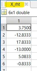
Substitute the values of X_rht matrix in equation (2) and find the second derivative using Right skew method.

Here, we observed that a=3.75; b=-12.8333; c=17.8333; d=-13; e=5.0833; g=-0.8333;

We find the coefficient, upto the term `f^(v)(i)dx^5`.

Divide `f^(vi)(i)dx^6`/ `dx^2`, we get the coefficient in the order of `dx^4`. We are neglecting that terms, so we can say that our approximation is fourth order accurate.

SKEWED LEFT HAND DIFFERENCE SCHEME:

NO OF NODES:

The number of nodes = p+q

Where, p is order of derivative.

q is order of approximations.

The no of nodes = 2+4 =>6.

DERIVATION:

To derive a fourth order approximation for the second order derivative,we start with these approximation,

`frac(partial^2 y)(partial^2 x) = a*f(i-5)+b*f(i-4)+c*f(i-3)+d.f(i-2)+e*f(i-1)+g*f(i)` --------------(3)

expand all the terms in the equation (2) using taylor series expansion and are represented in the form of table using taylor table method.

`dx^2*f''(i)`	`f(i)`	`f'(i)*dx`	`f''(i)*dx^2`	`f'''(i)dx^3`	`f^(iv)(i)dx^4`	`f^(v)(i)dx^5`	`f^(vi)(i)dx^6`
af(i-5)	a	-5a	25a/2	-125a/6	625a/24	-3125a/120	15625a/720
bf(i-4)	b	-4b	16b/2	-64b/6	256b/24	-1024b/120	4096b/720
cf(i-3)	c	-3c	9c/2	-27c/6	81c/24	-243c/120	729c/720
df(i-2)	d	-2d	4d/2	-8d/6	16d/24	-32d/120	64d/720
ef(i-1)	e	-e	e/2	-e/6	e/24	-e/120	e/720
gf(i)	g	0	0	0	0	0	0
Sum of Coefficient	0	0	1	0	0	0

the linear equation obtained from the above table are solved using matrix inversion method,

A.X = B

A= `[[1,1,1,1,1,1],[-5,-4,-3,-2,-1,0],[25/2,16/2,9/2,4/2,1/2,0],[-125/6,-64/6,-27/6,-8/6,-1/6,0],[625/24,256/24,81/24,16/24,1/24,0],[-3125/120,-1024/120,-243/120,-32/120,-1/120,0]]`;

X=`[[a],[b],[c],[d],[e],[g]]`;

B= `[[0],[0],[1],[0],[0],[0]]`;

X=A\B;

We get X as shown below

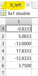
Substitute the values of X_left matrix in equation (3) and find the second derivative using Right skew method.

Here, we observed that a=-0.8333; b=5.0833; c=-13; d=17.8333; e=-12.8333; f=3.75;

We find the coefficient, upto the term `f^(v)(i)dx^5`.

Divide `f^(vi)(i)dx^6`/ `dx^2`, we get the coefficient in the order of `dx^4`. We are neglecting that terms, so we can say that our approximation is fourth order accurate.

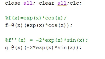
f(x) is the function given in question and g(x) is its analytic second derivative.

Now define the value of x at which the derivative to be calculated and also define the range of dx

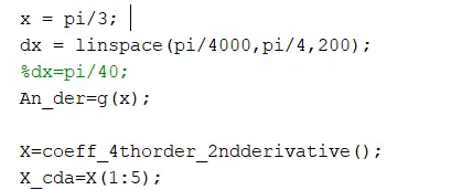
dx can be grid size or step size. As the value of dx is small, the more accurate the solution.

X=coeff_4thorder_2ndderivative(); This means accessing the values in the function coeff_4thorder_2ndderivative();

coeff_4thorder_2ndderivative() have all the coefficient values of all the 3 schemes that we used here.

Accessing Coefficients of Central difference scheme is shown below

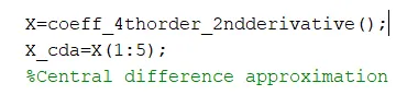
Use the variable cd to calculate values of second derivative in Central difference scheme;

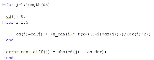
The variable error_cent_diff is used to find the absolute value of error between analytical method and Central difference scheme.

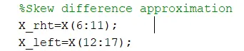
X_rht and X_left are the coefficients of right and left skew respectively.

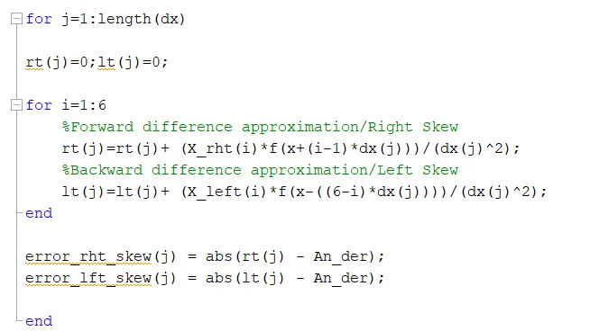
Use the variable rt and lt to calculate values of second derivative in right and left skew respectively;

The variable error_rht_skew and error_lft_skew are used to find the absolute value of error between analytical method and right and left skew respectively.

Now, plot the error vs dx in normal scale

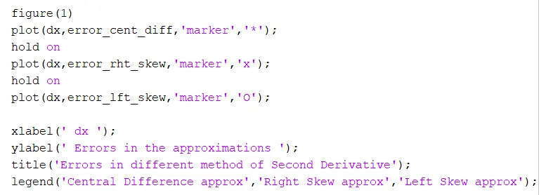
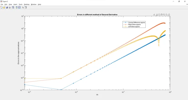
Now, plot the error vs dx in logarithmic scale

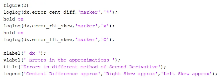
Now, lets move to the function to calculate the coefficients in all the 3 schemes

A,B,X are the matrix explained above in theory.

The term cda is added to A,B,X to indicate that it is Central difference scheme.

The term fda is added to A,B,X to indicate that it is Forward difference scheme/Right Skew method.

The term bda is added to A,B,X to indicate that it is Backward difference scheme/Left Skew method.

The variable X is used to store all the coefficients of CDA,FDA(Right Skew) and BDA(Left Skew) methods.

MATLAB program

close all; clear all;clc;

%f(x)=exp(x)*cos(x);
f=@(x)(exp(x)*cos(x));

%f''(x) = -2*exp(x)*sin(x);
g=@(x)(-2*exp(x)*sin(x));


x = pi/3; 
dx = linspace(pi/4000,pi/4,200);
%dx=pi/40;
An_der=g(x);

X=coeff_4thorder_2ndderivative();
X_cda=X(1:5);
%Central difference approximation

for j=1:length(dx)

cd(j)=0;
for i=1:5
    
    cd(j)=cd(j) + (X_cda(i)* f(x-((3-i)*dx(j))))/(dx(j)^2);
end

error_cent_diff(j) = abs(cd(j) - An_der);
end
%Skew difference approximation
X_rht=X(6:11);              
X_left=X(12:17);

for j=1:length(dx)

rt(j)=0;lt(j)=0;

for i=1:6
    %Forward difference approximation/Right Skew
    rt(j)=rt(j)+ (X_rht(i)*f(x+(i-1)*dx(j)))/(dx(j)^2);
    %Backward difference approximation/Left Skew
    lt(j)=lt(j)+ (X_left(i)*f(x-((6-i)*dx(j))))/(dx(j)^2);
end

error_rht_skew(j) = abs(rt(j) - An_der);
error_lft_skew(j) = abs(lt(j) - An_der);

end

figure(1)
plot(dx,error_cent_diff,'marker','*');
hold on
plot(dx,error_rht_skew,'marker','x');
hold on
plot(dx,error_lft_skew,'marker','O');

xlabel(' dx ');
ylabel(' Errors in the approximations ');
title('Errors in different method of Second Derivative');
legend('Central Difference approx','Right Skew approx','Left Skew approx');

figure(2)
loglog(dx,error_cent_diff,'marker','*');
hold on
loglog(dx,error_rht_skew,'marker','x');
hold on
loglog(dx,error_lft_skew,'marker','O');

xlabel(' dx ');
ylabel(' Errors in the approximations ');
title('Errors in different method of Second Derivative');
legend('Central Difference approx','Right Skew approx','Left Skew approx');


figure(3)
plot(dx,cd,'marker','*');
hold on
plot(dx,rt,'marker','x');
hold on
plot(dx,lt,'marker','O');
hold on
plot(dx,An_der,'--','marker','x');

xlabel(' dx ');
ylabel(' Second Derivative ');
title('Second Derivative values Vs dx');
legend('Central Difference approx','Right Skew approx','Left Skew approx','Analytical result');


figure(4)
loglog(dx,cd,'marker','*');
hold on
loglog(dx,rt,'marker','x');
hold on
loglog(dx,lt,'marker','O');
hold on
loglog(dx,An_der,'marker','square');

xlabel(' dx ');
ylabel(' Second Derivative ');
title('Second Derivative values Vs dx');
legend('Central Difference approx','Right Skew approx','Left Skew approx','Analytical result');

Function to get coefficients

function [X] = coeff_4thorder_2ndderivative()


A_cda=[1,1,1,1,1;  -2,-1,0,1,2;  4/2,1/2,0,1/2,4/2;  -8/6,-1/6,0,1/6,8/6;  16/24,1/24,0,1/24,16/24];

B_cda=[0;0;1;0;0];
X_cda=A_cda\B_cda;


A_fda=[1,1,1,1,1,1;  0,1,2,3,4,5;  0,1/2,4/2,9/2,16/2,25/2;  0,1/6,8/6,27/6,64/6,125/6;  0,1/24,16/24,81/24,256/24,625/24;  0,1/120,32/120,243/120,1024/120,3125/120];
B_fda=[0;0;1;0;0;0];
X_fda=A_fda\B_fda;


A_bda=[1,1,1,1,1,1;  -5,-4,-3,-2,-1,0;  25/2,16/2,9/2,4/2,1/2,0;  -125/6,-64/6,-27/6,-8/6,-1/6,0;  625/24,256/24,81/24,16/24,1/24,0;  -3125/120,-1024/120,-243/120,-32/120,-1/120,0];
B_bda=[0;0;1;0;0;0];
X_bda=A_bda\B_bda;

X=[X_cda;X_fda;X_bda];

end

OUTPUT

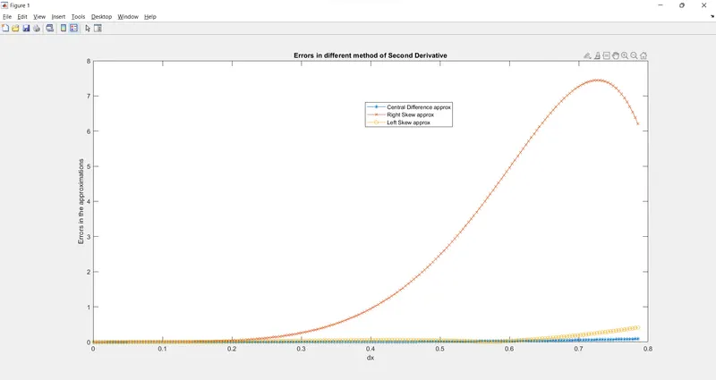
a) Error in normal scale

b) Error in logarithmic scale

Explanation of output

As the mesh size or step size(dx) increases, the error increases. The central difference scheme is found to be more accurate of small mesh size(within range).

CD uses information from both the sides from the point of consideration to give approximative and accurate values.

As the left and right skewed difference methods uses data only from one side of point of interest it gives less approximative and accurate values about the point.

In your own words, describe why a skewed scheme is useful? What can a skewed scheme do that a CD scheme cannot?

The CD scheme is useful inside a domain and it gives more accurate results than the skewed schemes and we found it from the graph. The mesh size or step size(dx) should be within a particular range.

If the system doesn’t contain sufficient information on both side of the point of interest, we cannot use central differencing scheme so skewed scheme is useful in such cases.

CDS cannot not be employed at the boundary nodes due to unavailability of right and left nodes at the same time. In such cases the skewed differencing scheme is used.

At the boundary, the skewed schemes are useful.

At left side of the control volume, right skew method is suitable.

At right side of the control volume, left skew method is suitable.