Week 3.5 - Deriving 4th order approximation of a 2nd order derivative using Taylor Table method

AIM :

• To derive the Fourth Order Approximations of the Second Order Derivative using matlab.
• Central Differencing.
• Skewed Right Side Difference.
• Skewed Left Side Difference.

OBJECTIVES :

• To evaluate the Second Order Derivative of the analytical function `exp(x)*cos(x)` and compare it with three numerical approximations.
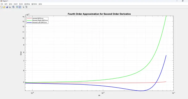
• To plot the absolute error for the given datas.
• The order of accuracy P = Number of nodes in the stencil N - order of derivative Q + 1 for symmetric/central schemes
• The order of accuracy P = Number of nodes in the stencil N - order of derivative Q for one-sided/skewed schemes
• To Solve the system of equations using the matrix inversion method in Matlab to obtain the taylor table coefficients and use them directly in the numerical approximation statements to avoid input errors.

PROCEDURE :

CENTRAL DIFFERENCING SCHEME.

In applied mathematics, the central differencing scheme is a finite difference method that optimizes the approximation for the differential operator in the central node of the considered patch and provides numerical solutions to differential equations. In central differencing the points have been taken on both sides respectively.

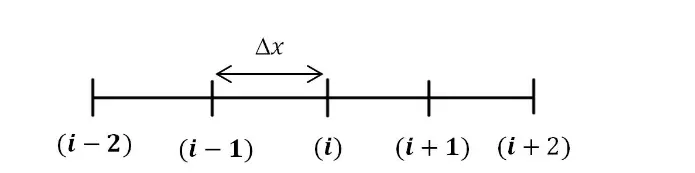
• Order of Accuracy = P
• Number of Nodes in Stencils = N
• Order of Derivatives = Q

NUMBER OF STENCILS N = P+Q -1

N = 2 + 4 -1

N = 6-1

N = 5.

Second Order Derivation for fourth Order Approximation.

`(del^2 u )/(delx^2) = a f_((i-2)) +b f_(( i-1)) +c f_(( i)) +d f _(( i+1)) + e f_((i+2))`

Taylor series expansion.

`af_((i-2)) = af((i)) - (2af'(i)dx)/(1!) + (4af''(i)dx^2)/(2!) -(8af'''(i)dx^3)/(3!) +(16af''''(i)dx^4)/(4!)`+......

`bf(i-1) = bf(i) -(bf'(i)dx)/(1!)+(bf''(i)dx^2)/(2!)-(bf'''(i)dx^3)/(3!)+(bf''''(i)dx^4)/(4!)`

`cf(i) = cf(i)`

`df(i+1) = df(i) +(df'(i)dx)/(1!)+(df''(i)dx^2)/(2!)+(df'''(i)dx^3)/(3!)+(df''''(i)dx^4)/(4!)`

`ef_((i+2)) = ef((i)) + (2ef'(i)dx)/(1!) + (4ef''(i)dx^2)/(2!) +(8ef'''(i)dx^3)/(3!) +(16ef''''(i)dx^4)/(4!)`

TAYLOR TABLE.

`dx^2 f''(i)`	`f(i)`	`f'(i)dx`	`f''(i) dx^2`	`f'''(i)dx^3`	`f''''(i)dx^4`
`a f_((i-2))`	a	-2a	4a/2	-8a/6	16a/24
`b f_((i-1))`	b	-b	b/2	-b/6	b/24
`c f _((i))`	c	0	0	0	0
`df_((i+1))`	d	d	d/2	d/6	d/24
`e f_((i+2))`	e	2e	4e/2	8e/6	16e/24
sum of co_efficients	0	0	1	0	0

`a +b + c +d +e = 0` ....... eqn 1 .

`(-2a) +(-b) + d +2e = 0` ........eqn 2.

`(4a)/2 +(b)/2 +(d)/2 +(4e)/2 = 1` .........eqn 3.

`(-8a)/6 +(-b)/6 +(d)/6 +(8e)/6 = 0` ..........eqn 4.

`(16a)/24 +(b)/24 +(d)/24+(16e)/24 = 0` ...........eqn 5.

With the help of taylor table method linear equation is obtained. let us convert in the matrix form.

A*X = B

`[[1,1,1,1,1],[-2,-1,0,1,2],[4/2,1/2,0,1/2,4/2],[-8/6,-1/6,0,1/6,8/6],[16/24,1/24,0,1/24,16/24]]*[[a],[b],[c],[d],[e]]` = `[[0],[0],[1],[0],[0]]`

X = inv(A)*B

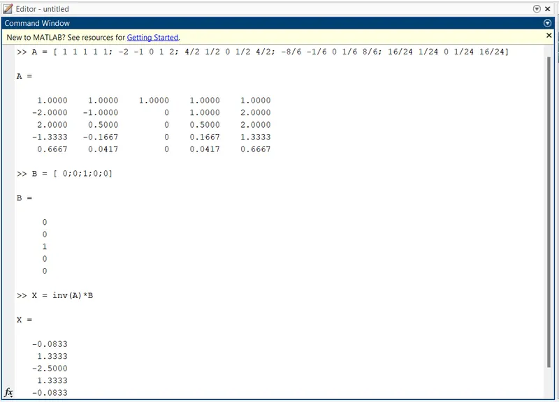
• a = - 0.0833
• b = 1.3333
• c = -2.5000
• d = 1.3333
• e = -0.0833

Final equation.

`(del^2u)/(delx^2) =( (-0.0833)f(i-2)+(1.3333)f(i-1)+(-2.5000)f(i)+(1.3333)f(i+1) +(-0.0833)f(i+2))/(dx^2)`

SKEWED RIGHT HAND DIFFERENCING SCHEME.

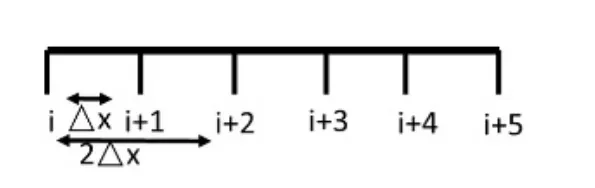
• Order of Accuracy = P
• Number of Nodes in Stencils = N
• Order of Derivatives = Q

NUMBER OF STENCILS N = P+Q

N = 2+4

N = 6

SECOND ORDER DERIVATION.

`(del^2u)/(delx^2) = a f(i) +bf(i+1) + c f(i+2) +d f(i+3) +e f(i+4) +g f(i+5)`

TAYLOR TABLE.

`dx^2f''(i)`	`f(i)`	`f'(i)dx`	`f''(i)dx^2`	`f'''(i)dx^3`	`f''''(i)dx^4`	`f'''''(i)dx^5`
af(i)	a	0	0	0	0	0
bf(i+1)	b	b	b/2	b/6	b/24	b/120
cf(i+2)	c	2c	4c/2	8c/6	16c/24	32c/120
df(i+3)	d	3d	9d/2	27d/6	81d/24	243d/120
ef(i+4)	e	4e	16e/2	64e/6	256e/24	1024e/120
gf(i+5)	g	5g	25g/2	125g/6	625g/24	3125g/120
sum of co_efficients	0	0	1	0	0	0

`a + b+ c+ d + e + g = 0` ..............eqn 1.

`b+2c+3d+4e+5g =0` ..............eqn 2.

`(b/2) + (4c)/(2) +(9d)/(2) + (16e)/(2) + (25g)/(2) = 0` ..............eqn 3.

`(b/6) + (8c)/(6) +(27d)/(6) +(64e)/(6) +(125g)/(6) = 0` ...............eqn 4.

`(b)/24 +(16c)/24+(81d)/24 +(256e)/24 +(625g)/24 = 0` ................eqn 5.

`(b/120) + (32c)/120 +(243d)/120 +(1024e)/120 +(3125g)/120 = 0` ................eqn 6.

with the help of taylor table method, Six equation and Six unknown let us converted into matrix form and find the values respectively.

A*X = B

`[[1, 1, 1, 1,1,1],[0,1,2,3,4,5],[0,1/2,4/2,9/2,16/2,25/2],[0,1/6,8/6,27/6,64/6,125/6],[0,1/24,16/24,81/24,256/24,625/24],[0 ,1/20,32/120,243/120, 1024/120, 3125/120]] *[[a],[b],[c],[d],[e],[g]]` = `[[0],[0],[1],[0],[0],[0]]`

X = inv(A)*B

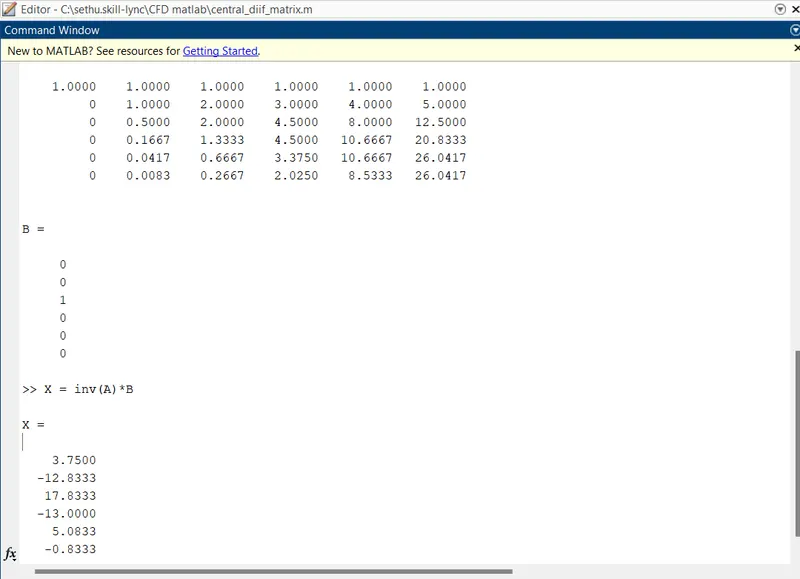
• a = 3.7500
• b = -12.8333
• c = 17.8333
• d = -13.0000
• e = 5.0833
• g = -0.8333

Final equation.

`(del^2u) /(delx^2) = ((3.7500)f(i) +(-12.8333)f(i+1)+(17.8333)f(i+2)+(-13.0000)f(i+3)+(5.0833)f(i+4)+(-0.8333)f(i+5))/dx^2`

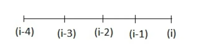
SKEWED LEFT HAND DIFFERENCING SCHEME.

• Order of Accuracy = P
• Number of Nodes in Stencils = N
• Order of Derivatives = Q

NUMBER OF STENCILS N = P+Q

N = 2+4

N = 6

SECOND ORDER DERIVATION.

`(del^2u)/delx^2 = af(i-5) +bf(i-4) + cf(i-3) +df(i-2) +ef(i-1)+g(i)` `

TAYLOR TABLE.

`dx^2 f''(i)`	`f(i)`	`f'(i)dx`	`f''(i) dx^2`	`f'''(i)dx^3`	`f''''(i) dx^4`	`f'''''(i)dx^5`
af(i-5)	a	-5a	25a/2	-125a/6	625a/24	-3125a/120
bf(i-4)	b	-4b	16b/2	-64b/6	256b/24	-1024b/120
cf(i-3)	c	-3c	9c/2	-27c/6	81c/24	-243c/120
df(i-2)	d	-2d	4d/2	-8d/6	16d/24	-32d/120
ef(i-1)	e	-1e	e/2	-e/2	e/24	-e/120
gf(i)	g	0	0	0	0	0
sum of co_efficients	0	0	1	0	0	0

`a + b+ c + d + e + g = 0 ......eqn 1`

`(-5a ) + (-4b) + (-3c) + (-2d) + (-1e) = 0 ......eqn2`

`(25a)/2 +(16b)/2+(9c)/2 +(4d)/2 +(e)/2 = 1 ......eqn3`

`(-125a)/6 +(-64b)/6 +(-27c)/6+(-8d)/6+(-e)/6 =0 .....eqn4`

`(625a)/24 +(256b)/24 +(81c)/24 +(16d)/24 + (e)/24 = 0 .......eqn5`

`(-3125a)/120 + (-1024b)/120 +(-243c)/120+(-32d)/120+(-e)/120 = 0`......eqn6.

A*X = B

`[[ 1,1,1,1,1,1],[-5,-4,-3,-2,-1,0],[25/2,16/2,9/2,4/2,1/2,0],[-125/6,-64/6,-27/6,-8/6,-1/6,0],[625/24,256/24,81/24,16/24,1/24,0],[-3125/120,-1024/120,-243/120,-32/120,-1/20,0]]*[[a],[b],[c],[d],[e],[g]] = [[0],[0],[1],[0],[0],[0]]`

X = inv(A)*B

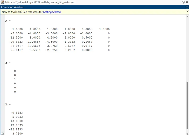
• a = - 0.8333
• b = 5.0833
• c = -13.0000
• d = 17.8333
• e = -12.8333
• g = 3.7500

Final equation.

`(del^2u)/(delx^2) =( (-0.8333)f(i-5) + (5.0833)f(i-4)+(-13.0000)f(i-3)+(17.8333)f(i-2) +(-12.8333)f(i-1) +(3.7500)f(i))/dx^2`

clear all 
close all 
clc 

% central differencing linear matrix 

 A = [ 1 1 1 1 1; -2 -1 0 1 2; 4/2 1/2 0 1/2 4/2; -8/6 -1/6 0 1/6 8/6; 16/24 1/24 0 1/24 16/24];

 B = [ 0;0;1;0;0];

 X = inv(A)*B


% skewed right hand differencing linear matrix 

A = [1 1 1 1 1 1; 0 1 2 3 4 5; 0 1/2 4/2 9/2 16/2 25/2; 0 1/6 8/6 27/6 64/6 125/6; 0 1/24 16/24 81/24 256/24 625/24;0 1/120 32/120 243/120 1024/120 3125/120]
B = [0; 0; 1; 0; 0; 0]

X = inv(A)*B 

%  Skewed left hand differencing linear  matrix 

A = [1 1 1 1 1 1; -5 -4 -3 -2 -1 0; 25/2 16/2 9/2 4/2 1/2 0; -125/6 -64/6 -27/6 -8/6 -1/6 0; 625/24 256/24 81/24 16/24 1/24 0; -3125/120 -1024/120 -243/120 -32/120 -1/120 0]
B = [0;0;1;0;0;0]

X = inv(A)*B    

MAIN PROGRAM.

% Solving fourth order approximation for Second order derivative

clear all 
close all 
clc 

% Inputs 
% x value 
x = pi/3;

% dx range 
dx = linspace(pi/4000,pi/40,20);

% for loop method 

for i = 1:length(dx)

    central_difference_error(i) = fourth_order_central_differencing(x,dx(i));
    skewed_right_hand_difference_error(i) = skewed_right_hand_differencing(x,dx(i));
    skewed_left_hand_difference_error(i) = skewed_left_hand_differencing(x,dx(i));

end 


% plotting 

loglog(dx,central_difference_error,'color','r','linewidth',1)
hold on 
loglog(dx,skewed_right_hand_difference_error,'color','g','linewidth',1.5)
hold on
loglog(dx,skewed_left_hand_difference_error,'color','b','linewidth',2)
title('Fourth Order Approximation for Second Order Derivative','FontSize',14)
xlabel('dx','FontSize',10)
ylabel('Error','FontSize',10)
legend('Central Diff Error','Skewed Right Diff Error','Skewed Left Diff Error','location','northwest')
grid on 

FUNCTION CODE.

• Inline function is used (that is ) @(x)
• Instead of i term x is replaced and for constant terms dx is replaced.

FUNCTION FOR CENTRAL DIFFERENCING.

function [out_1] = fourth_order_central_differencing(x,dx)

% Analytical function 
% f(x) = exp(x)*cos(x)

% Analytical derivative 
% f'(x) = exp(x)*cos(x)-exp(x)*sin(x)
% for second order derivative 
% f''(x) = -2*exp(x)*sin(x)

f = @(x) exp(x)*cos(x);

% Analytical derivative 
analytical_derivative = -2*exp(x)*sin(x);

% Numerical derivative
% central_differencing = ((-0.0833)f(x-2dx)+(1.3333)f(x-dx)+(-2.5000)f(x)+(1.3333)f(x+dx)+(-0.0833)f(x+2dx))/(dx^2);

% Numerical derivative 
central_differencing = ((-0.0833)*f(x-2*dx)+(1.3333)*f(x-dx)+(-2.5000)*f(x)+(1.3333)*f(x+dx)+(-0.0833)*f(x+2*dx))/(dx^2);
  
% errors 
out_1 = abs(central_differencing-analytical_derivative);

end 

FUNCTION FOR SKEWED RIGHT HAND DIFFERENCING.

function [out_2] = skewed_right_hand_differencing(x,dx)


% Analytical function 
% f(x) = exp(x)*cos(x)

% Analytical derivative 
% f'(x) = exp(x)*cos(x)-exp(x)*sin(x)
% for second order derivative 
% f''(x) = -2*exp(x)*sin(x)

f = @(x) exp(x)*cos(x);

% Analytical derivative 
analytical_derivative = -2*exp(x)*sin(x); 

% Numerical derivative
% skewed_right_hand_differencing =
% ((3.7500)f(x)+(-12.8333)f(x+dx)+(17.8333)f(x+2dx)+(-13.0000)f(x+3dx)+(5.0833)f(x+4dx)+(-0.8333)f(x+5dx))/(dx^2)

% Numerical derivative 
skewed_right_differencing = ((3.7500)*f(x)+(-12.8333)*f(x+dx)+(17.8333)*f(x+2*dx)+(-13.0000)*f(x+3*dx)+(5.0833)*f(x+4*dx)+(-0.8333)*f(x+5*dx))/(dx^2);

% errors
out_2 = abs(skewed_right_differencing-analytical_derivative);

end

FUNCTION FOR SKEWED LEFT HAND DIFFERENCING.

function [out_3]= skewed_left_hand_differencing(x,dx)

% Analytical function 
% f(x) = exp(x)*cos(x)

% Analytical derivative 
% f'(x) = exp(x)*cos(x)-exp(x)*sin(x)
% for second order derivative 
% f''(x) = -2*exp(x)*sin(x)

f = @(x) exp(x)*cos(x);

% Analytical derivative 
analytical_derivative = -2*exp(x)*sin(x);

% Numerical derivative 
% skewed_left_hand_difference =
% ((-0.8333)f(x-5dx)+(5.0833)f(x-4dx)+(-13.0000)f(x-3dx)+(17.8333)f(x-2dx)+(-12.8333)f(x-dx)+(3.7500)f(x))/(dx^2);

% Numerical derivative 
skewed_left_differencing = ((-0.8333)*f(x-5*dx)+(5.0833)*f(x-4*dx)+(-13.0000)*f(x-3*dx)+(17.8333)*f(x-2*dx)+(-12.8333)*f(x-dx)+(3.7500)*f(x))/(dx^2);

% errors 
out_3 = abs(skewed_left_differencing-analytical_derivative);

end

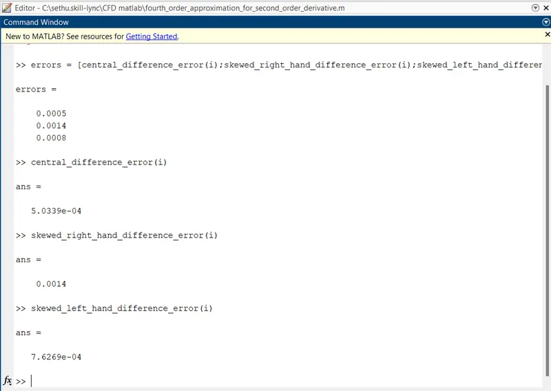
OUTPUT.

CODE EXPLANATION.

• The Program starts with clear all close all clc commands respectively.
• clear all command is used to clear the current workspace value whereas the close all command is used to close all the figure windows and finally clc command is uesd to clear the command window respectively.
• The given function that needed to be compute is f(x) = exp(x)*cos(x) with respect to the assuming input values of x = pi/3 ; dx= [pi/4000,pi/40]
• analytical derivative for f(x) = exp(x)*cos(x)
• first derivative `f'(x) = exp(x)*cos(x) - exp(x) *sin(x)`
• Second derivative `f''(x) = -2 *exp(x)*sin(x)`
• Inline function is used.
• Linspace command is used where the starting value and ending value and intervals given.
• for loop coomand is used to repeat the specific block of code a known number of times .
• finally plotting is done with the help of loglog.

USEFUL OF SKEWED SCHEME AND WHY CD SCHEME CANNOT.

• A skewed distribution is neither symmetric nor normal because the data values trail off more sharply on the one side than on the other.
• To calculate the value of function at boundary conditions Central Scheme cannot be used because it carries value at nodes on the both sides. In such a way skewed scheme is used.