Week 3.5 - Deriving 4th order approximation of a 2nd order derivative using Taylor Table method
Deriving 4th order approximation of a 2nd order derivative using the Taylor Table method
AIM:
1. To derive the following 4th-order approximations of the second-order derivative.
1. Central difference
2. Skewed right-sided difference
3. Skewed left-sided difference
2. To write a program in Matlab to evaluate the second-order derivative of the analytical function exp(x)*cos(x) and compare it with the 3 numerical approximations.
PROCEDURE:
1. Central difference:
The order of accuracy P = Number of nodes in the stencil N - order of derivative Q + 1 for symmetric/central schemes
The number of nodes in the stencil (N )=The order of accuracy (P )+order of derivative (Q ) -1 for symmetric/central schemes.
Therefore the number of nodes to be considered for a 4th-order accurate approximation of a second-order derivative by the central difference method is given by:
N=4+2-1=5
To derive a fourth order approximation for the second order derivative, we start with this approximation,
`Delta x^2( (del^2 u)/(delx^2))=af(i-2)+bf(i-1)+cf(i)+df(i+1)+ef(i+2)`
TAYLOR'S TABLE:
| `f(i)` | `Delta x f'(i)` | `Delta x^2 f''(i)` | `Delta x^3 f(i)'''` | `Delta x^4 f''''(i)` | `Delta x^5 f'''''(i)` | `Delta x^6 f''''''(i)` | |
| af(i-2) | a | -2a | 4a/2 | -8a/6 | 16a/24 | -32a/120 | 64a/240 |
| bf(i-1) | b | -b | b/2 | -b/6 | b/24 | -b/120 | b/240 |
| cf(i) | c | 0 | 0 | 0 | 0 | 0 | 0 |
| df(i+1) | d | d | d/2 | d/6 | d/24 | d/120 | d/240 |
| ef(i+2) | e | 2e | 4e/2 | 8e/6 | 16e/24 | 32e/120 | 64e/240 |
| `Delta x^2 f''(x)` | 0 | 0 | 1 | 0 | 0 | ? | ? |
since we are trying to compute second-order derivative the only term we should have on the right-hand side is f''(x) which means the sum of columns in the table for the first 2 columns should be equal to 0 and the third column =1 and 4th and 5th column =0 ,sixth and seventh column unknown and in the original hypothesis we have 5 unknowns which means we need only 5 equations to solve the system and remaining what they sum up to we don't know we just ignore higher order terms Since only the second derivative of the function is to be found out, the sum of the coefficients of `f’’(i) (dx)^2` alone equal to 1 and the rest all are zero.
`af(i-2)=a(f(i)-(2Delta x) f'(i)+(2Delta x)^2/(2! )f''(i)-(2Delta x)^3/(3! )f'''(i)+(2Delta x)^4/(4! )f''''(i))`
`bf(i-1)=b(f(i)-Delta x f'(i)+Delta x^2/(2! )f''(i)-Delta x^3/(3! )f'''(i)+Delta x^4/(4! )f''''(i))`
`cf(i)=cf(i)`
`df(i+1)=d(f(i)+Delta x f'(i)+Delta x^2/(2! )f''(i)+Delta x^3/(3! )f'''(i)+Delta x^4/(4! )f''''(i))`
`ef(i+2)=e(f(i)+(2Delta x) f'(i)+(2Delta x)^2/(2! )f''(i)+(2Delta x)^3/(3! )f'''(i)+(2Delta x)^4/(4! )f''''(i))`
a+b+c+d+e =0
-2a-b+0+d+2e = 0
4a/2+b/2 +0+d/2+4e/2= 1
-8a/6-b/6+0+d/6+8e/6 =0
16a/24+b/24+0+d/24+16e/24=0
The linear equation obtained from the above table is solved using the matrix inversion method,
A.X = B
`[[1,1,1,1,1],[-2,-1,0,1,2],[4/2,1/2,0,1/2,4/2],[-8/6,-1/6,0,1/6,8/6],[16/24,1/24,0,1/24,16/24]].[[a],[b],[c],[d],[e]] = [[0],[0],[1],[0],[0]]`
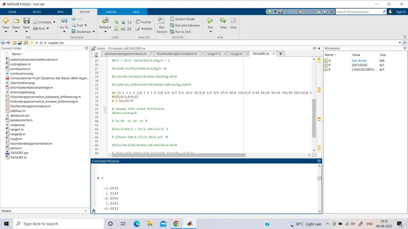
X = inv(A)*B
-0.0833
1.3333
-2.5000
1.3333
-0.0833
`(del^2u)/(delx^2) = ((-0.0833)f(i-2)+(1.3333)f(i-1)+(-2.5000)f(i)+(1.3333)f(i+1)+(-0.0833)f(i+2))/(∆x^2)`
2. Skewed right-sided difference:
The order of accuracy (P )= Number of nodes in the stencil (N )- order of derivative (Q ) for one-sided/skewed schemes.
The number of nodes in the stencil (N )=The order of accuracy (P )+order of derivative (Q ) for one-sided/skewed schemes.
Therefore the number of nodes to be considered for a 4th-order accurate approximation of a second-order derivative by the Skewed right-sided method is given by:
N=4+2=6
To derive a fourth order approximation for the second order derivative, we start with this approximation,
`Delta x^2( d^2u)/(dx^2)=af(i)+bf(i+1)+cf(i+2)+df(i+3)+ef(i+4)+gf(i+5)`
TAYLOR'S TABLE:
| `f(i)` | `Delta x f'(i)` | `Delta x^2 f''(i)` | `Delta x^3 f(i)'''` | `Delta x^4 f''''(i)` | `Delta x^5 f'''''(i)` | `Delta x^6 f''''''(i)` | |
| af(i) | a | 0 | 0 | 0 | 0 | 0 | 0 |
| bf(i+1) | b | b | b/2 | b/6 | b/24 | b/120 | b/720 |
| cf(i+2) | c | 2c | 4c/2 | 8c/6 | 16c/24 | 32c/120 | 64c/720 |
| df(i+3) | d | 3d | 9d/2 | 27d/6 | 81d/24 | 243d/120 | 729d/720 |
| ef(i+4) | e | 4e | 16e/2 | 64e/6 | 256e/24 | 1024e/120 | 4096e/720 |
| gf(i+5) | g | 5g | 25g/2 | 125g/6 | 625g/24 | 3125g/120 | 15625g/720 |
| `Delta x^2 f''(x)` | 0 | 0 | 1 | 0 | 0 | 0 | ? |
since we are trying to compute second-order derivative the only term we should have on the right-hand side is f''(x) which means the sum of columns in the table for the first 2 columns should be equal to 0 and the third column =1 and 4th and 5th column =0 ,sixth column unknown and in the original hypothesis we have 6 unknowns which means we need only 6 equations to solve the system and remaining what they sum up to we don't know we just ignore higher order terms Since only the second derivative of the function is to be found out, the sum of the coefficients of `f’’(i) (dx)^2` alone equal to 1 and the rest all are zero.
We get 6 coupled algebraic equations for 6 unknowns ignoring the higher order terms in Taylor's table.
`af(i)=af(i)`
`bf(i+1)=b(f(i)+Delta x f'(i)+Delta x^2/(2! )f''(i)+Delta x^3/(3! )f'''(i)+Delta x^4/(4! )f''''(i)+Delta x^5/(5!) f'''''(i))`
`cf(i+2)=c(f(i)+(2Delta x) f'(i)+(2Delta x)^2/(2! )f''(i)+(2Delta x)^3/(3! )f'''(i)+(2Delta x)^4/(4! )f''''(i)+(2Delta x)^5/(5!) f'''''(i))`
`df(i+3)=d(f(i)+(3Delta x) f'(i)+(3Delta x)^2/(2! )f''(i)+(3Delta x)^3/(3! )f'''(i)+(3Delta x)^4/(4! )f''''(i)+(3Delta x)^5/(5!) f'''''(i))`
`ef(i+4)=e(f(i)+(4Delta x) f'(i)+(4Delta x)^2/(2! )f''(i)+(4Delta x)^3/(3! )f'''(i)+(4Delta x)^4/(4! )f''''(i)+(4Delta x)^5/(5!) f'''''(i))`
`gf(i+5)=d(f(i)+(5Delta x) f'(i)+(5Delta x)^2/(2! )f''(i)+(5Delta x)^3/(3! )f'''(i)+(5Delta x)^4/(4! )f''''(i)+(5Delta x)^5/(5!) f'''''(i))`
a+b+c+d+e+g =0
b+2c+3d+4e+5g = 0
b/2 + 4c/2 +9d/2+16e/2+25g/2 = 1
b/6+8c/6+27d/6+64e/6+125g/6 =0
b/24+16c/24+81d/24+256e/24+625g/24=0
b/120+32c/120+243d/120+1024e/120+3125g/120=0
The linear equation obtained from the above table is solved using the matrix inversion method,
A.X = B
`[[1,1,1,1,1,1],[0,1,2,3,4,5],[0,1/2,4/2,9/2,16/2,25/2],[0,1/6,8/6,27/6,64/6,125/6],[0,1/24,16/24,81/24,256/24,625/24],[0,1/120,32/120,243/120,1024/120,3125/120]].[[a],[b],[c],[d],[e],[g]] = [[0],[0],[1],[0],[0],[0]]`
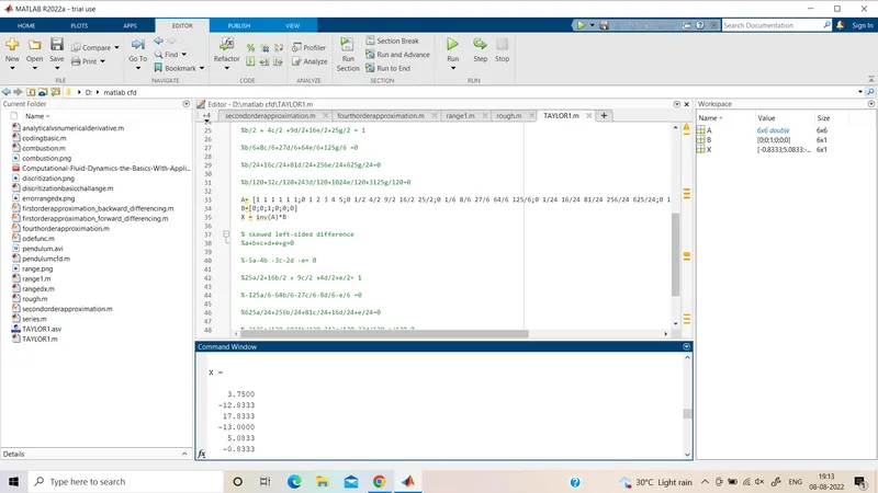
X = inv(A)*B
X =
3.7500
-12.8333
17.8333
-13.0000
5.0833
-0.8333
proof of skewed right scheme is fourth-order accurate:
rewriting equations in terms of Taylor series expansion of individual terms by substituting the coefficient values of a, b, c, d,e, g leads to:
`(del^2 u)/(delx^2) =(a+b+c+d+e+g)f(i)+(b+2c+3d+4e+5g) f ' (i)∆x+(b/2+(4c)/2+(9d)/2+(16e)/2+(25g)/2) f '' (i) ∆x^2+(b/6+(8c)/6+(27d)/6+(64e)/6+(125g)/6) f''' (i) ∆x^3+(b/24+(16c)/24+(81d)/24+(256e)/24+(625g)/24) f'''' (i) ∆x^4+(b/120+(32c)/120+(243d)/120+(1024e)/120+(3125g)/120) f''''' (i) ∆x^5+(b/720+(64c)/720+(729d)/720+(4096e)/720+(15625g)/720) f'''''' (i) ∆x^6`
`Delta x^2( (del^2 u)/(delx^2))=af(i)+bf(i+1)+cf(i+2)+df(i+3)+ef(i+4)+gf(i+5)`
`af(i)+bf(i+1)+cf(i+2)+df(i+3)+ef(i+4)+gf(i+5)`=`(b/2+(4c)/2+(9d)/2+(16e)/2+(25g)/2) f '' (i) ∆x^2+O(∆x^4)`
dividing both side by
`Deltax^2`
`(del^2 f)/(delx^2) ≅`(af(i)+bf(i+1)+cf(i+2)+df(i+3)+ef(i+4)+gf(i+5))/(∆x^2)`=(b/2+(4c)/2+(9d)/2+(16e)/2+(25g)/2) f '' (i) ∆x^2+O(∆x^4)`
`O(∆x^4):`truncation error of 4th order`
`(del^2 f)/(delx^2) ≅( 3.75* f(i) -12.8333*f(i+1) + 17.8333*f(i+2)-13.0000*f(i+3) +5.0833*f(i+4) -0.8333*f(i+5))/(∆x^2)`
3. Skewed left-sided difference:
The order of accuracy (P )= Number of nodes in the stencil (N )- order of derivative (Q ) for one-sided/skewed schemes.
The number of nodes in the stencil (N )=The order of accuracy (P )+order of derivative (Q ) for one-sided/skewed schemes.
Therefore the number of nodes to be considered for a 4th-order accurate approximation of a second-order derivative by the Skewed right-sided method is given by:
N=4+2=6
To derive a fourth order approximation for the second order derivative, we start with this approximation,
`Delta x^2( (del^2 u)/(delx^2))=af(i-5)+bf(i-4)+cf(i-3)+df(i-2)+ef(i-1)+gf(i)`
TAYLOR'S TABLE:
| `f(i)` | `Delta x f'(i)` | `Delta x^2 f''(i)` | `Delta x^3 f(i)'''` | `Delta x^4 f''''(i)` | `Delta x^5 f'''''(i)` | Delta x^6 f''''''(i) | |
| af(i-5) | a | -5a | 25a/2 | -125a/6 | 625a/24 | -3125a/120 | 15625a/720 |
| bf(i-4) | b | - 4b | 16b/2 | -64b/6 | 256b/24 | -1024b/120 | 4096b/720 |
| cf(i-3) | c | - 3c | 9c/2 | -27c/6 | 81c/24 | -243c/120 | 729c/720 |
| df(i-2) | d | - 2d | 4d/2 | -8d/6 | 16d/24 | -32d/120 | 64d/720 |
| ef(i-1) | e | -e | e/2 | -e/6 | e/24 | -e/120 | e/720 |
| gf(i) | g | 0 | 0 | 0 | 0 | 0 | 0 |
| `Delta x^2 f''(x)` | 0 | 0 | 1 | 0 | 0 | 0 | ? |
`af(i-5)=a(f(i)-(5Delta x) f'(i)+(5Delta x)^2/(2! )f''(i)-(5Delta x)^3/(3! )f'''(i)+(5Delta x)^4/(4! )f''''(i)-(5Delta x)^5/(5!) f'''''(i))`
`bf(i-4)=b(f(i)-(4Delta x) f'(i)+(4Delta x)^2/(2! )f''(i)-(4Delta x)^3/(3! )f'''(i)+(4Delta x)^4/(4! )f''''(i)-(4Delta x)^5/(5!) f'''''(i))`
`cf(i-3)=c(f(i)-(3Delta x) f'(i)+(3Delta x)^2/(2! )f''(i)-(3Delta x)^3/(3! )f'''(i)+(3Delta x)^4/(4! )f''''(i)-(3Delta x)^5/(5!) f'''''(i))`
`df(i-2)=d(f(i)-(2Delta x) f'(i)+(2Delta x)^2/(2! )f''(i)-(2Delta x)^3/(3! )f'''(i)+(2Delta x)^4/(4! )f''''(i)-(2Delta x)^5/(5!) f'''''(i))`
`ef(i-1)=e(f(i)-Delta x f'(i)+Delta x^2/(2! )f''(i)-Delta x^3/(3! )f'''(i)+Delta x^4/(4! )f''''(i)-Delta x^5/(5!) f'''''(i))`
`gf(i)=gf(i)`
since we are trying to compute second-order derivative the only term we should have on the right-hand side is f''(x) which means the sum of columns in the table for the first 2 columns should be equal to 0 and the third column =1 and 4th and 5th column =0 , sixth column unknown and in the original hypothesis we have 6 unknowns which means we need only 6 equations to solve the system and remaining what they sum up to we don't know we just ignore higher order terms Since only the second derivative of the function is to be found out, the sum of the coefficients of `f’’(i) (dx)^2` alone equal to 1 and the rest all are zero.
We get 6 coupled algebraic equations for 6 unknowns ignoring the higher order terms in Taylor's table.
a+b+c+d+e+g=0
-5a-4b -3c-2d -e= 0
25a/2+16b/2 + 9c/2 +4d/2+e/2= 1
-125a/6-64b/6-27c/6-8d/6-e/6 =0
625a/24+256b/24+81c/24+16d/24+e/24=0
-3125a/120-1024b/120-243c/120-32d/120-e/120=0
The linear equation obtained from the above table is solved using the matrix inversion method,
A.X = B
`[[1,1,1,1,1,1],[-5,-4,-3,-2,-1,0],[25/2,16/2,9/2,4/2,1/2,0],[-125/6,-64/6,-27/6,-8/6,-1/6,0],[625/24,256/24,81/24,16/24,1/24,0],[-3125/120,-1024/120,-243/120,-32/120,-1/120,0]].[[a],[b],[c],[d],[e],[g]] = [[0],[0],[1],[0],[0],[0]]`
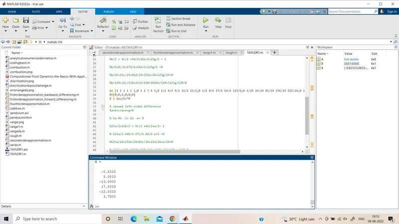
X =
-0.8333
5.0833
-13.0000
17.8333
-12.8333
3.7500
proof of skewed left scheme is fourth-order accurate:
similarly as skewed right scheme (we can see that the absolute values of constants are the same just in reverse order)
`af(i-5)+bf(i-4)+cf(i-3)+df(i-2)+ef(i-1)+gf(i)`=`((25a)/2+(16b)/2+(9c)/2+(4d)/2+(e)/2) f '' (i) ∆x^2+O(∆x^4)`
dividing both side by
`Deltax^2`
`(del^2 f)/(delx^2) ≅``(af(i-5)+bf(i-4)+cf(i-3)+df(i-2)+ef(i-1)+gf(i))/(Deltax^2)`=`((25a)/2+(16b)/2+(9c)/2+(4d)/2+(e)/2 f '' (i) ∆x^2+O(∆x^4)`
`(del^2 f)/(delx^2) ≅(-0.8333f(i-5)+5.0833f(i-4)-13.0000f(i-3)+17.8333f(i-2)-12.8333f(i-1)+3.7500f(i))/(∆x^2)`
Thus,skewed schemes are fourth-order accurate(proved).
PROGRAM TO FIND TAYLOR TABLE COEFFICIENTS: the matrix inversion method in Matlab to obtain the Taylor table coefficients
clear all
close all
clc
%central difference

%a+b+c+d+e =0

%-2a-b+0+d+2e = 0

%4a/2+b/2 +0+d/2+4e/2= 1

%-8a/6-b/6+0+d/6+8e/6 =0

%16a/24+b/24+0+d/24+16e/24=0

A= [1 1 1 1 1 ;-2 -1 0 1 2;4/2 1/2 0 1/2 4/2 ;-8/6 -1/6 0 1/6 8/6;16/24 1/24 0 1/24 16/24]
B=[0;0;1;0;0]
X = inv(A)*B

% skewed right-sided difference
%a+b+c+d+e+g =0

%b+2c+3d+4e+5g = 0

%b/2 + 4c/2 +9d/2+16e/2+25g/2 = 1

%b/6+8c/6+27d/6+64e/6+125g/6 =0

%b/24+16c/24+81d/24+256e/24+625g/24=0

%b/120+32c/120+243d/120+1024e/120+3125g/120=0

A= [1 1 1 1 1 1;0 1 2 3 4 5;0 1/2 4/2 9/2 16/2 25/2;0 1/6 8/6 27/6 64/6 125/6;0 1/24 16/24 81/24 256/24 625/24;0 1/120 32/120 243/120 1024/120 3125/120]
B=[0;0;1;0;0;0]
X = inv(A)*B

% skewed left-sided difference
%a+b+c+d+e+g=0

%-5a-4b -3c-2d -e= 0

%25a/2+16b/2 + 9c/2 +4d/2+e/2= 1

%-125a/6-64b/6-27c/6-8d/6-e/6 =0

%625a/24+256b/24+81c/24+16d/24+e/24=0

%-3125a/120-1024b/120-243c/120-32d/120-e/120=0

A= [1 1 1 1 1 1;-5 -4 -3 -2 -1 0;25/2 16/2 9/2 4/2 1/2 0;-125/6 -64/6 -27/6 -8/6 -1/6 0;625/24 256/24 81/24 16/24 1/24 0;-3125/120 -1024/120 -243/120 -32/120 -1/120 0]
B=[0;0;1;0;0;0]
X = inv(A)*B
PROCEDURE:
STEP-1:Firstly we’re going to write programs to develop functions for central, skewed right-sided, and skewed left-sided errors at a particular point (x, dx), where dx represents spacing in between each node. These functions will help us to calculate errors over the range of ‘dx’. With the help of code ‘function out we’re going to make a function; which we save in the directory and call according to our need in the main program.
function out1=centraldifference(x,dx)

% analytical_function f(x)=exp(x)*cos(x);
% f'(x)=-exp(x)*sin(x)+exp(x)*cos(x);
% f''(x)=-2*exp(x)*sin(x)


analytical_derivative=-2*exp(x)*sin(x)


% values of coefficients calculated from our Taylor table;

a=-0.0833;
b=1.3333;
c=-2.5000;
d=1.3333;
e=-0.0833;


% numerical_derivative
%af(i-2)+bf(i-1)+cf(i)+df(i+1)+ef(i+2)
% central_differencing=((a*f(x-2*dx)+b*f(x-1*dx)+c*f(x)+d*f(x+dx)+ef(x+2*dx))/dx^2
central_differencing=((a*exp(x-2*dx)*cos(x-2*dx))+(b*exp(x-1*dx)*cos(x-1*dx))+(c*exp(x)*cos(x))+(d*exp(x+1*dx)*cos(x+1*dx))+(e*exp(x+2*dx)*cos(x+2*dx)))/dx^2

out1=abs(central_differencing-analytical_derivative)

end
function out2=skewedrightsideddifference(x,dx)
% analytical_function f(x)=exp(x)*cos(x);
% f'(x)=-exp(x)*sin(x)+exp(x)*cos(x);
% f''(x)=-2*exp(x)*sin(x)
analytical_derivative=-2*exp(x)*sin(x)
% values of coefficients calculated from our Taylor table;
a=3.7500;
b=-12.8333
c=17.8333;
d=-13.0000;
e=5.0833;
g=-0.8333;
% numerical_derivative
%af(i)+bf(i+1)+cf(i+2)+df(i+3)+ef(i+4)+gf(i+5)
%skewedright_differencing=((a*f(x))+(b*f(x+1*dx)+(c*f(x+2*dx)+(d*f(x+3*dx)+(e*f(x+4*dx)+(g*f(x+5*dx)))/dx^2
skewedright_differencing=((a*exp(x)*cos(x))+(b*exp(x+1*dx)*cos(x+1*dx))+(c*exp(x+2*dx)*cos(x+2*dx))+(d*exp(x+3*dx)*cos(x+3*dx))+(e*exp(x+4*dx)*cos(x+4*dx))+(g*exp(x+5*dx)*cos(x+5*dx)))/dx^2
out2=abs(skewedright_differencing-analytical_derivative)
endfunction out3=skewedleftsideddifference(x,dx)
% analytical_function f(x)=exp(x)*cos(x);
% f'(x)=-exp(x)*sin(x)+exp(x)*cos(x);
% f''(x)=-2*exp(x)*sin(x)
analytical_derivative=-2*exp(x)*sin(x)
% values of coefficients calculated from our Taylor table;
a=-0.8333;
b=5.0833
c=-13.0000;
d=17.8333;
e=-12.8333;
g=3.7500;
% numerical_derivative
%af(i-5)+bf(i-4)+cf(i-3)+df(i-2)+ef(i-1)+gf(i)
%skewedleft_differencing=((a*f(x-5*dx)+b*f(x-4*dx)+c*f(x-3*dx)+d*f(x-2*dx)+ef(x-1*dx)+gf(x))/dx^2
skewedleft_differencing=((a*exp(x-5*dx)*cos(x-5*dx))+(b*exp(x-4*dx)*cos(x-4*dx))+(c*exp(x-3*dx)*cos(x-3*dx))+(d*exp(x-2*dx)*cos(x-2*dx))+(e*exp(x-1*dx)*cos(x-1*dx))+(g*exp(x)*cos(x)))/dx^2
out3=abs(skewedleft_differencing-analytical_derivative)
endSTEP-2:
After creating the above functions, we save our main program in the same directory in which we have saved our three functions:centraldifference,skewedrightsideddifference,skewedleftsideddifference
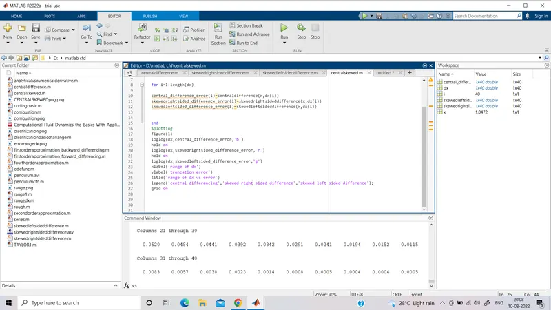
For now, we’re going to create an array for the range of ‘dx’. We’ll use ‘for loop’ over the range of ‘dx’ and using the functions centraldifference,skewedrightsideddifference,skewedleftsideddifference 4th order error at a given point (x, dx), we’ll get the errors for a range of ‘dx’ and also we’re going to plot the graph between ‘error’ vs. ‘dx’ for central, skewed right-sided, and skewed left-sided difference 4th order error.
PROGRAMMING:
clear all
close all
clc
%range of dx
x=pi/3;
dx=linspace(pi/4,pi/40000,40)

for i=1:length(dx)

central_difference_error(i)=centraldifference(x,dx(i))
skewedrightsided_difference_error(i)=skewedrightsideddifference(x,dx(i))
skewedleftsided_difference_error(i)=skewedleftsideddifference(x,dx(i))


end
%plotting
figure(1)
loglog(dx,central_difference_error,'b')
hold on
loglog(dx,skewedrightsided_difference_error,'r')
hold on
loglog(dx,skewedleftsided_difference_error,'g')
xlabel('range of dx')
ylabel('truncation error')
title('range of dx vs error')
legend('central differencing','skewed right sided difference','skewed left sided difference');
grid on
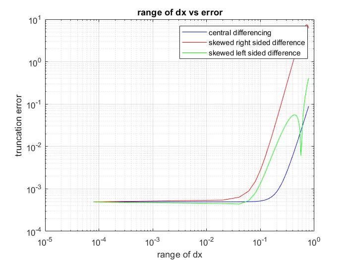
After analyzing the graph between ‘error’ vs. ‘range of dx’ for central, skewed right-sided, and skewed left-sided difference 4th order error; we can easily notice that central difference approximation produces more accurate solutions; hence produces lesser errors as compared to right-skewed and left-skewed difference schemes.
A skewed scheme is useful: a skewed scheme does that a CD scheme cannot
The central differencing scheme gives us lesser errors as compared to the skewed difference scheme but it is not always viable to use the central differencing to evaluate solutions. In some cases, a skewed difference scheme is more useful than compared to the central difference.
Suppose, if we want to compute numerical approximations for a function at the boundary or corner node; we cannot use the central difference scheme in this particular situation because it requires data from both sides of the node or boundary. So, in this situation skewed difference method plays a major role; as in the skewed scheme data from one side can be used to compute numerical approximation at a point.