Week 3.5 - Deriving 4th order approximation of a 2nd order derivative using Taylor Table method

AIM:-

Derive the following 4th order approximations of the second-order derivative.

1. Central difference

2. Skewed right-sided difference

3. Skewed left-sided difference

DERIVATION :-

1. Central difference

The numerical stencil for central Difference Scheme is

(i-2)-----------(i-1)-----------(i)-----------(i+1)-----------(i+2)

For central difference scheme the double derivative can be written as follows

`(d^2y)/(dx^2)=af(i-2)+bf(i-1)+cf(i)+df(i+1)+ef(i+2)` ------(1)

Using Taylor Series we can expand the above equation as follows,

`af(i-2)=a(f(i)-2Deltaxf'(i)+((2Deltax)^2f''(i))/(2!)-((2Deltax)^3f'''(i))/(3!)+((2Deltax)^4foverset(iv) .(i))/(4!))`

`bf(i-1)=b(f(i)-Deltaxf'(i)+((Deltax)^2f''(i))/(2!)-((Deltax)^3f'''(i))/(3!)+((Deltax)^4foverset(iv) .(i))/(4!))`

`cf(i)=c`

`df(i+1)=d(f(i)+Deltaxf'(i)+((Deltax)^2f''(i))/(2!)+((Deltax)^3f'''(i))/(3!)+((Deltax)^4foverset(iv) .(i))/(4!))`

`ef(i+2)=e(f(i)+2Deltaxf'(i)+((2Deltax)^2f''(i))/(2!)+((2Deltax)^3f'''(i))/(3!)+((2Deltax)^4foverset(iv) .(i))/(4!))`

from the taylor Table the value of the coefficient can be found,

	`f(i)`	`Deltaxf'(i)`	`Deltax^2f''(i)`	`Deltax^3f'''(i)`	`Deltax^4foverset(iv).(i)`
`af(i-2)`	a	-2a	`(4a)/2`	`(-8a)/6`	`(16a)/24`
`bf(i-1)`	b	-b	`b/2`	`(-b)/6`	`b/24`
`cf(i)`	c	0	0	0	0
`df(i+1)`	d	d	`d/2`	`d/6`	`d/24`
`ef(i+2)`	e	2e	`(4e)/2`	`(8e)/6`	`(16e)/24`
sum	0	0	1	0	0

From above taylor table we get following equations

a+b+c+d+e=0

-2a-b+d+2e=0

4a/2+b/2+d/2+4e/2=1

-8a/6-b/6+d/6+8e/6=0

16a/24+b/24+d/24+32e/24=0

the above equations can be solved in matrix by converting to matrix form .

A1=[1 1 1 1 1;-2 -1 0 1 2 ;2 0.5 0 0.5 2;-4/3 -1/6 0 1/6 4/3; 2/3 1/24 0 1/24 2/3]

B1=[0;0;1;0;0]

X1=[a;b;c;d;e]

Consider A1X1=B1

by solving above equation in matlab we get,

a= -0.0833

b= 1.3333

c=-2.5000

d=1.3333

e=-0.0833

Hence a=e,b=d

equation (1) becomes

`f''(i)=(af(i-2)+bf(i-1)+cf(i)+df(i+1)+ef(i+2))/(Deltax^2)`

The order of accuracy P = Number of nodes in the stencil N - order of derivative Q + 1

number of nodes = 5 ( a,b,c,d,e) | order of derivative = 2 ( second order derivative `(d^2y)/dx^2` )

The order of accuracy P = 5-2+1

The order of accuracy P = 4 . so its fourth order approximation

2. Skewed right hand scheme :

The numerical stencil for Skewed Right hand Scheme is

(i)-----------(i+1)-----------(i+2)-----------(i+3)-----------(i+4)-----------(i+5)

For Skewed Right hand scheme the double derivative can be written as follows

`(d^2y)/dx^2=af(i)+bf(i+1)+cf(i+2)+df(i+3)+ef(i+4)+gf(i+5)` ------(2)

Using Taylor Series we can expand the above equation as follows,

`bf(i+1)=b(f(i)+Deltaxf'(i)+((Deltax)^2f''(i))/(2!)+((Deltax)^3f'''(i))/(3!)+((Deltax)^4foverset(iv) .(i))/(4!)+((Deltax)^5foverset(v).(i))/(5!))`

`cf(i+2)=c(f(i)+2Deltaxf'(i)+((2Deltax)^2f''(i))/(2!)+((2Deltax)^3f'''(i))/(3!)+((2Deltax)^4foverset(iv) .(i))/(4!)+((2Deltax)^5foverset(v).(i))/(5!))`

`df(i+3)=d(f(i)+3Deltaxf'(i)+((3Deltax)^2f''(i))/(2!)+((3Deltax)^3f'''(i))/(3!)+((3Deltax)^4foverset(iv) .(i))/(4!)+((3Deltax)^5foverset(v).(i))/(5!))`

`ef(i+4)=e(f(i)+4Deltaxf'(i)+((4Deltax)^2f''(i))/(2!)+((4Deltax)^3f'''(i))/(3!)+((4Deltax)^4foverset(iv) .(i))/(4!)+((4Deltax)^5foverset(v).(i))/(5!))`

`gf(i+5)=g(f(i)+5Deltaxf'(i)+((5Deltax)^2f''(i))/(2!)+((5Deltax)^3f'''(i))/(3!)+((5Deltax)^4foverset(iv) .(i))/(4!)+((5Deltax)^5foverset(v).(i))/(5!))`

from the taylor Table the value of the coefficient can be found,

	`f(i)`	`Deltaxf'(i)`	`Deltax^2f''(i)`	`Deltax^3f'''(i)`	`Deltax^4foverset(iv).(i)`	`Deltax^5foverset(v).(i)`
`af(i)`	a	0	0	0	0	0
`bf(i+1)`	b	b	`b/2`	`(b)/6`	`b/24`	`b/120`
`cf(i+2)`	c	2c	`(4c)/2`	`(8c)/6`	`(16c)/24`	`(32c)/120`
`df(i+3)`	d	3d	`(9d)/2`	`(27d)/6`	`(81d)/24`	`(243d)/120`
`ef(i+4)`	e	4e	`(16e)/2`	`(64e)/6`	`(256e)/24`	`(1024e)/120`
`gf(i+5)`	g	5g	`(25g)/2`	`(125g)/6`	`(625g)/24`	`(3125g)/120`
sum	0	0	1	0	0	0

we get following equation from taylor table

a+b+c+d+e+g=0

b+2c+3d+4e+5g=0

b/2+4c/2+9d/2+16e/2+25g/2=1

b/6+8c/6+27d/6+64e/6+125g/6=0

b/24+16c/24+81d/24+256e/24+625g/24=0

b/120+32c/120+243d/120+1024e/120+3125g/120=0

the above equations can be solved in matrix by converting to matrix form .

Consider A2X2=B2

by solving above equation in matlab we get,

a=3.7500

b= -12.8333

c=17.8333

d=-13.0000

e=5.0833

g=-0.8333

We have

`f''(i)=(af(i)+bf(i+1)+cf(i+2)+df(i+3)+ef(i+4)+gf(i+5))/(Deltax^2)`

The order of accuracy P = Number of nodes in the stencil N - order of derivative Q

number of nodes = 6 ( a,b,c,d,e,g) | order of derivative = 2 ( second order derivative `(d^2y)/dx^2` )

The order of accuracy P = 6-2

The order of accuracy P = 4 . so its fourth order approximation

3. Skewed left hand scheme :

The numerical stencil for Skewed left hand Scheme is

(i-5)-----------(i-4)-----------(i-3)-----------(i-2)-----------(i-1)-----------(i)

For Skewed left hand scheme the double derivative can be written as follows

`(d^2y)/dx^2=af(i-5)+bf(i-4)+cf(i-3)+df(i-2)+ef(i-1)+gf(i)`-------(3)

Using Taylor Series we can expand the above equation as follows,

`af(i-5)=a(f(i)-5Deltaxf'(i)+((5Deltax)^2f''(i))/(2!)-((5Deltax)^3f'''(i))/(3!)+((5Deltax)^4foverset(iv) .(i))/(4!)-((5Deltax)^5foverset(v).(i))/(5!))`

`bf(i-4)=b(f(i)-4Deltaxf'(i)+((4Deltax)^2f''(i))/(2!)-((4Deltax)^3f'''(i))/(3!)+((4Deltax)^4foverset(iv) .(i))/(4!)-((4Deltax)^5foverset(v).(i))/(5!))`

`cf(i-3)=c(f(i)-3Deltaxf'(i)+((3Deltax)^2f''(i))/(2!)-((3Deltax)^3f'''(i))/(3!)+((3Deltax)^4foverset(iv) .(i))/(4!)-((3Deltax)^5foverset(v).(i))/(5!))`

`df(i-2)=d(f(i)-2Deltaxf'(i)+((2Deltax)^2f''(i))/(2!)-((2Deltax)^3f'''(i))/(3!)+((2Deltax)^4foverset(iv) .(i))/(4!)-((2Deltax)^5foverset(v).(i))/(5!))`

`ef(i-1)=e(f(i)-Deltaxf'(i)+((Deltax)^2f''(i))/(2!)-((Deltax)^3f'''(i))/(3!)+((Deltax)^4foverset(iv) .(i))/(4!)-((Deltax)^5foverset(v).(i))/(5!))`

from the taylor Table the value of the coefficient can be found,

	`f(i)`	`Deltaxf'(i)`	`Deltax^2f''(i)`	`Deltax^3f'''(i)`	`Deltax^4foverset(iv).(i)`	`Deltax^5foverset(v).(i)`
`af(i-5)`	a	-5a	`(25a)/2`	`(-125a)/6`	`(625a)/24`	`(-3125a)/120`
`bf(i-4)`	b	-4b	`(16b)/2`	`(-64b)/6`	`(256b)/24`	`(-1024b)/120`
`cf(i-3)`	c	-3c	`(9c)/2`	`(-27c)/6`	`(81c)/24`	`(-243c)/120`
`df(i-2)`	d	-2d	`(4d)/2`	`(-8d)/6`	`(16d)/24`	`(-32d)/120`
`ef(i-1)`	e	-e	`e/2`	`(-e)/6`	`e/24`	`(-e)/120`
`gf(i)`	g	0	0	0	0	0
sum	0	0	1	0	0	0

we get following equation from taylor table

a+b+c+d+e+g=0

-5a-4b-3c-2d-e=0

25a/2+16b/2+9c/2+4d/2+e/2=1

-125a/6-64b/6-27c/6-8d/6-e/6=0

625a/24+256b/24+81c/24+16d/24+e/24=0

-3125a/120-1024b/120-243c/120-32d/120-e/120=0

we can solve above equations by converting to matrix form

Consider A3X3=B3

by solving above equation in matlab we get,

a=-0.8333

b= 5.0833

c=-13.0000

d=17.8333

e=-12.8333

g=3.7500

we have

`f''(i)=(af(i-5)+bf(i-4)+cf(i-3)+df(i-2)+ef(i-1)+gf(i))/(Deltax^2)`

The order of accuracy P = Number of nodes in the stencil N - order of derivative Q

number of nodes = 6 ( a,b,c,d,e,g) | order of derivative = 2 ( second order derivative `(d^2y)/dx^2` )

The order of accuracy P = 6-2

The order of accuracy P = 4 . so its fourth order approximation

MATLAB CODE :-

close all
clear all
clc

x= pi/3;
dx= linspace(pi/4, pi/400,100);
% analytical function = exp(x)*cos(x)

% analytical second derivative 
analytical_second_derivative = -2*exp(x)*sin(x);

%% calculating coefficients 

% central difference scheme 
A1=[1 1 1 1 1;-2 -1 0 1 2 ;2 1/2 0 1/2 2;-4/3 -1/6 0 1/6 4/3; 2/3 1/24 0 1/24 2/3];
B1=[0;0;1;0;0];
X1=linsolve(A1,B1);

a1= X1(1);
b1= X1(2);
c1= X1(3);
d1= X1(4);
e1= X1(5);

% Skewed right hand scheme 
A2=[1 1 1 1 1 1;0 1 2 3 4 5;0 1/2 4/2 9/2 16/2 25/2;0 1/6 8/6 27/6 64/6 125/6;0 1/24 16/24 81/24 256/24 625/24;0 1/120 32/120 243/120 1024/120 3125/120;];
B2=[0;0;1;0;0;0];
X2=linsolve(A2,B2);

a2= X2(1);
b2= X2(2);
c2= X2(3);
d2= X2(4);
e2= X2(5);
g2= X2(6);

% Skewed left hand scheme
A3=[1 1 1 1 1 1;-5 -4 -3 -2 -1 0;25/2 16/2 9/2 4/2 1/2 0;-125/6 -64/6 -27/6 -8/6 -1/6 0;625/24 256/24 81/24 16/24 1/24 0;-3125/120 -1024/120 -243/120 -32/120 -1/120  0];
B3=[0;0;1;0;0;0];
X3=linsolve(A3,B3);

a3= X3(1);
b3= X3(2);
c3= X3(3);
d3= X3(4);
e3= X3(5);
g3= X3(6);

%% numerical derivative 

central_diff = (a1.*exp(x-2.*dx).*cos(x-2.*dx)+b1.*exp(x-dx).*cos(x-dx)+c1.*exp(x).*cos(x)+d1.*exp(x+dx).*cos(x+dx)+e1.*exp(x+2.*dx).*cos(x+2.*dx))./((dx).^2);
skewed_right = (a2.*exp(x).*cos(x)+b2.*exp(x+dx).*cos(x+dx)+c2.*exp(x+2.*dx).*cos(x+2.*dx)+d2.*exp(x+3.*dx).*cos(x+3.*dx)+e2.*exp(x+4.*dx).*cos(x+4.*dx)+g2.*exp(x+5.*dx).*cos(x+5.*dx))./((dx).^2);
skewed_left =  (a3.*exp(x-5.*dx).*cos(x-5.*dx)+b3.*exp(x-4.*dx).*cos(x-4.*dx)+c3.*exp(x-3.*dx).*cos(x-3.*dx)+d3.*exp(x-2.*dx).*cos(x-2.*dx)+e3.*exp(x-dx).*cos(x-dx)+g3.*exp(x).*cos(x))./((dx).^2);

%% error

error_central = abs(analytical_second_derivative - central_diff);
error_right = abs(analytical_second_derivative - skewed_right);
error_left = abs(analytical_second_derivative - skewed_left);

%% plot 

loglog(dx,error_central,'linewidth',3)
hold on
loglog(dx,error_right,'linewidth',3)
hold on 
loglog(dx,error_left,'linewidth',3)
xlabel('dx')
ylabel('Absolute error')
legend('central difference scheme','skewed right hand scheme','skewed left hand scheme')

• first we define the input conditions like x and dx .
• analytical second order derivative is calculated.
• next we solve the equations we have got from taylor table . we convert the equations into matrix form ( AX=B ) and solve it by matrix inversion method .
• here linsolve function helps us to solve these equations .
• next numerical derivative for different schemes is calculated by substituting the coefficients obtained for various constants in their respective equations .
• error is calculated for all 3 schemes by taking absolute value of difference between analytical second order derivative and numerical derivative .
• we use loglog to plot the results .

RESULTS :-

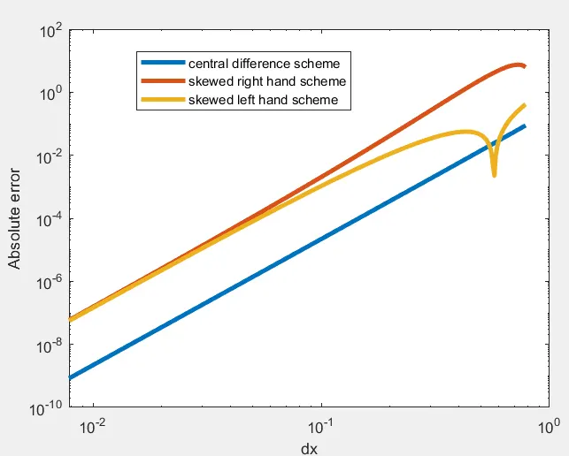
• we are limiting the x axix . reducing dx too much will result in rounding off values and results in increasing the error .
• The above graph shows that for the value of dx the central difference scheme gives the very less error as compared to the Skewed right and skewed left hand difference scheme.CDS utilizes the available information from left and right ie both the sides.
• The error decreasing rate for Skewed right and Central Difference scheme is same but for skewed left hand scheme it is comparatively low
• In skewed scheme the information used is from right and left side from successive neighbouring points there error occur is higher than all other scheme.Skewed scheme is used to compute higher order approximation.
• when we take the slope for each lines we find , slope of skewed right > slope of skewed left > slope of central difference .
• so we can say that skewed right hand scheme has high error rate while central differencing scheme has low error rate .

CONCLUSION :-

We have successfully run program in Matlab to evaluate the second-order derivative of the analytical function exp(x)*cos(x) and compare it with the 3 numerical approximations .