Week 3 - Solving second order ODEs
SOLVING SECOND ORDER ODEs
AIM:-
- Program that solves the ODE which represents the equation of motion of a simple pendulum with damping.
- Program to simulate pendulum motion
THEORY:-
Simple harmonic motion :
Simple Harmonic Motion or SHM is defined as a motion in which the restoring force is directly proportional to the displacement of the body from its mean position. The direction of this restoring force is always towards the mean position.A pendulum in simple harmonic motion is called a simple pendulum. A pendulum has an object with a small mass, also known as the pendulum bob, which hangs from a light wire or string. The equilibrium position for a pendulum is where the angle θθ">θ is zero (that is, when the pendulum is hanging straight down).
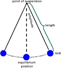
Damping is an influence within or upon an oscillatory system that has the effect of reducing or preventing its oscillation. In physical systems, damping is produced by processes that dissipate the energy stored in the oscillation.
GOVERNING EQUATIONS
Simple pendulum with damping equation
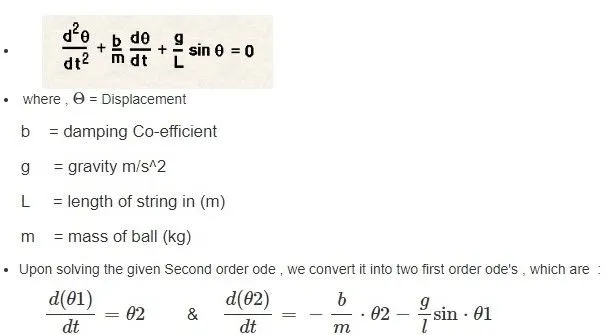
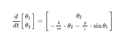
`d/dt[theta1;theta2]=d/dt[theta]`
in matlab program for representing `d/dttheta` we use 'dtheta_dt'. we represent similarly for other terms too.
CODE
1. function for solving the ODE
% function for finding solution for ODE equation
function[dtheta_dt]=ode_func(t,theta,b,g,l,m)

    theta1 = theta(1);
    theta2 = theta(2);
    dtheta1_dt = theta2;
    dtheta2_dt = -(b/m)*theta2-(g/l)*sin(theta1);
    dtheta_dt = [dtheta1_dt;dtheta2_dt];
end
2. Program to solve ODE and simulate simple pendulum
% a program to solve ODE of simple pendulum with damping
% a program to simulate pendulum motion

clear all
close all
clc

% input data
b = 0.05; % damping coefficient
g = 9.81; % gravity
l = 1 ; % length of pendulam in m
m = 1 ; % mass in kg

% initial condition
% displacement = 0
% angular velocity = 3rad/s
theta_0 = [0;3];

% time points
t_span = linspace(0,20,500);

% solving ODE
[t,results] = ode45(@(t,theta) ode_func(t,theta,b,g,l,m),t_span ,theta_0);

figure(1)
plot(t,results(:,1))
hold on
plot(t,results(:,2))
ylabel('plot')
xlabel('time (in s)')
title('simple pendulam with damping')
legend('angular displacement','angular velocity')


ct=1;
for i=1:length(t)
a=results(i,1);
x0=0;
y0=0;
x1=l*sin(a);
y1=-l*cos(a); % It is -ve because point y1 lies in the -ve quadrant

figure(2)
plot([x0 x1],[y0 y1],'linewidth',3) % To plot the pendulum length
hold on
title('simulating simple pendulum')
plot([-1 1],[0 0]) % To plot the line on which the pendulum is fixed to
plot(x1,y1,'marker','.','markersize',50) % To plot the pendulum ball

axis([-2 2 -2 2])
hold off
% saving frames to array M
M(ct)=getframe(gcf);
ct=ct+1;
end

% creating video file
movie(M)
videofile=VideoWriter('Simple Pendulum.avi','uncompressed avi');
open(videofile)
writeVideo(videofile,M)
close(videofile)
STEPS:
1. we create a function ' ode_func' to solve the ode equation from the pendulum input . the equations for solving are given above in equation section.
2. in the main code , first we input the data for simple pendulum , like mass , length of pendulum string , damping coefficient , gravity ..
3. then we input initial conditions like angular velocity (3 rad/s) and time (20 sec)
4. then we solve the ode equation by 'ode45' function and calling the function 'ode_func'. 'ode_45' is an inbuilt first degree differential equation solver in matlab .
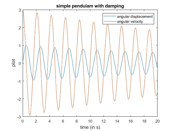
5. then we plot angular displacement and angular velocity against time with help of plot function.
6. with the help of for loop , we created many frames with different position of pendulum with time .
7. the created frames were stored in a array named M .
8. then we use movie command to created animation .
9. video file named ' simple_pendulum.avi' is created and we write the array M to the video file . this is done using 'VideoWriter' , 'writeVideo' functions of matlab
RESULT
plot:
simulation video of simple pendulum with damping :
CONCLUSION
ODE of equation of motion of simple pendulum with damping is solved and successfully created simulation video of simple pendulum with damping.