Week 3.5 - Deriving 4th order approximation of a 2nd order derivative using Taylor Table method

AIM:

• To Derive the following 4th order approximations of the second-order derivative of Central difference, Skewed right-sided difference, and skewed left-sided difference.
• To plot that compares the absolute error between the above-mentioned schemes.

CENTRAL DIFFERENCING SCHEME:

The No of Nodes = p+q-1 (Where p is the order of derivative & q is the order of approximations)

The No of Nodes = 2+4-1 = 5.

To derive a fourth-order approximation for the second-order derivative,

`(∂ ^2 u) /(∂ x^ 2) = (a f ( i-2 ) + b f ( i -1 ) + c f ( i ) + d f ( i +1 ) + e f ( i + 2 ) )/ (d x^2 )`.........(i)

`a f ( i − 2 ) = a f ( i ) − (2 a f ' ( i ) d x)/ (1 !) + (4 a f ' ' ( i ) d x ^2)/( 2 !) +( 8 a f ' ' ' ( i ) d x ^3) /(3 !) + (16 a f ' ' ' ' ( i ) d x ^4)/( 4 !)`

`dx^2f''(i)`	`f(i)`	`f'(i)dx`	`f''(i)dx^2`	`f'''(i)dx^3`	`f''''(i)dx^4`
af(i-2)	a	-2a	2a	`(-4a)/3`	`(2a)/3`
bf(i-1)	b	-b	`b/2`	`−b/6`	`b/24`
cf(i)	c	0	0	0	0
df(i+1)	d	d	`d/2`	`d/6`	`d/24`
ef(i+2)	e	2e	2e	`(4e)/3`	`(2e)/3`
Sum of Co-efficients	0	0	1	0	0

the linear equation obtained from the above table are solved using matrix inversion method,

`A.X=B`

`[[1 ,1,1,1,1],[-2,-1,0,1,2],[2,1/2,0,1/2,2], [-4/3,-1/6,0,1/6,4/3],[2/3,1/24,0,1/24,2/3]].[[a],[b],[c],[d],[e]]=[[0],[0],[1],[0],[0]]`

X = inv(A).B

So, a=-0.0833, b=1.3333, c=-2.5000, d=1.3333 e=-0.0833.

Sub the values of a,b,c,d,e in the Equation (i)

`(∂ ^2 u) /(∂ x^ 2) = (-0.0833 f ( i-2 ) + 1.3333 f ( i -1 ) -2.5 f ( i ) + 1.3333f ( i +1 ) -0.0833 f ( i + 2 ) )/ (d x^2 )``

SKEWED RIGHT-HAND DIFFERENCE SCHEME:

The N0 of Nodes = p+q (Where p is the order of derivative & q is the order of approximations)

The No of Nodes = 2+4 = 6.

`(∂ ^2 u) /(∂ x^ 2) = (a f ( i) + b f ( i +1 ) + c f ( i +2) + d f ( i +3 ) + e f ( i + 4)+gf(i+5) )/ (d x^2 )``.........(ii)

`dx^2f''(i)`	`f(i)`	`f'(i)dx`	`f''(i)dx^2`	`f'''(i)dx^3`	`f''''(i)dx^4`	`f'''''(i)dx^5`
af(i)	a	0	0	0	0	0
bf(i+1)	b	b	b/2	`b/6`	b/24	b/120
cf(i+2)	c	2c	4c/2	`(8c)/6`	16c/24	32c/120
df(i+3)	d	3d	9d/2	`(27d)/6`	81d/24	243d/120
ef(i+4)	e	4e	16e/2	`(64e)/6`	256e/24	1024e/120
gf(i+5)	g	5g	25g/2	`(125g)/6`	625g/24	3125g/120
Sum of Co-efficients	0	0	1	0	0	0

the linear equation obtained from the above table are solved using matrix inversion method,

A.X=B

`[[1 ,1,1,1,1,1],[0,1,2,3,4,5],[0,1/2,4/2,9/2,16/2,25/2], [0,1/6,8/6,27/6,64/6,125/6],[0,1/120,32/120,243/120,1024/120,3125/120]].[[a],[b],[c],[d],[e],[g]]=[[0],[0],[1],[0],[0],[0]]`

X = inv(A).B

So, a=3.7500, b=-12.8333, c=17.8333, d=-13.0000 e=5.0833 g=-0.8333.

Sub the values of a,b,c,d,e in the Equation (ii)

`(∂ ^2 u) /(∂ x^ 2) = (3.75 f ( i) -12.8333 f ( i +1 ) + 17.8333f ( i +2) + d f ( i +3 ) -13 f ( i + 4)+5.0833f(i+5) )/ (d x^2 )`

SKEWED LEFT-HAND DIFFERENCE SCHEME:

The No of Nodes = p+q (Where p is the order of derivative & q is the order of approximations)
The No of Nodes = 2+4 =6

`(∂ ^2 u) /(∂ x^ 2) = (a f ( i-5) + b f ( i -4) + c f ( i -3) + d f ( i -2 ) + e f ( i -1)+gf(i) )/ (d x^2 )`.............(iii)

`dx^2f''(i)`	`f(i)`	`f'(i)dx`	`f''(i)dx^2`	`f'''(i)dx^3`	`f''''(i)dx^4`	`f'''''(i)dx^5`
af(i-5)	a	-5a	`(25a)/2`	`(−125a)/6`	`(625a)/24`	`(−3125a)/120`
bf(i-4)	b	-4b	`(16b)/2`	`(-64b)/6`	`(256b)/24`	`(−1024b)/120`
cf(i-3)	c	-3c	`(9c)/2`	`(−27c)/6`	`(81c)/24`	`(−243c)/120`
df(i-2)	d	-2d	`(4d)/2`	`(−8d)/6`	`(16d)/24`	`(−32d)/120`
ef(i-1)	e	-e	`e/2`	`−e/6`	`e/24`	`−e/120`
gf(i)	g	0	0	0	0	0
Sum of Coefficients	0	0	1	0	0	0

the linear equation obtained from the above table are solved using the matrix inversion method,

A.X=B

`[[1 ,1,1,1,1,1],[-5,-4,-3,-2,-1,0],[25/2,16/2,9/2,4/2,1/2,0], [-125/6,-64/6,-27/6,-8/6,-1/6,0],[-3125/120,-1024/120,-243/120,-32/120,-1/120,0]].[[a],[b],[c],[d],[e],[g]]=[[0],[0],[1],[0],[0],[0]]`

X = inv(A).B

so, a=-0.8333, b=5.0833, c=-13.0000, d=17.8333 e=-12.8333 g=3.7500

Sub the values of a,b,c,d,e in the Equation (iii)

`(∂ ^2 u) /(∂ x^ 2) = (-0.8333 f ( i-5) + 5.0833 f ( i -4) -13 f ( i -3) + 17.8333 f ( i -2 ) -12.8333 f ( i -1)+9.75f(i) )/ (d x^2 )`

MAIN CODE:

clear all
close all
clc

%value of x
x= pi/3;

%range of dx
dx= linspace(pi/4,pi/4000,20);

%for loop
for i=1:length(dx)
    
    Central_Differencing(i) = fourth_order_central_differencing(x,dx(i));
    
    Right_Sided_Skew(i) = fourth_order_right_sided_skew(x,dx(i));
    
    Left_Sided_Skew(i) = fourth_order_left_sided_skew(x,dx(i));
    
end

%plotting
figure(1)
loglog(dx,Central_Differencing,'r')
hold on
loglog(dx,Right_Sided_Skew,'g')
hold on
loglog(dx,Left_Sided_Skew,'b')
grid on
xlabel('Range of dx')
ylabel('Absolute Error')
title('range of dx vs error')
legend('central differencing','skewed right sided difference','skewed left sided difference','location','northwest')

FUNCTION CODE FOR CENTRAL DIFFERENCING:

function Error_central_differencing = fourth_order_central_differencing(x,dx)

% analytic function = exp(x)*cos(x)

% analytic derivative
%f''(x) = -2*exp(x)*sin(x)

analytical_derivative = -2*exp(x)*sin(x);

%numerical derivative

%central differencing
central_differencing = (((-0.0833)*((exp(x-(2*dx)))*(cos(x-(2*dx)))))+((1.3333)*((exp(x-dx))*(cos(x-dx))))-((2.5000)*((exp(x))*(cos(x))))+((1.3333)*((exp(x+dx))*(cos(x+dx))))-((0.0833)*((exp(x+(2*dx)))*(cos(x+(2*dx))))))/(dx^2);

%error
Error_central_differencing = abs(central_differencing- analytical_derivative);
end

FUNCTION CODE FOR SKEWED RIGHT SIDED DIFFERENCE:

function Error_right_sided_skew = fourth_order_right_sided_skew(x,dx)

% analytic function = exp(x)*cos(x)

% analytic derivative
%f''(x) = -2*exp(x)*sin(x)

analytical_derivative = -2*exp(x)*sin(x);

%numerical derivative

%central differencing
right_sided_skew = (((3.7500)*((exp(x))*(cos(x))))-((12.8333)*((exp(x+dx))*(cos(x+dx))))+((17.8333)*((exp(x+(2*dx)))*(cos(x+(2*dx)))))-((13.0000)*((exp(x+(3*dx)))*(cos(x+(3*dx)))))+((5.0833)*((exp(x+(4*dx)))*(cos(x+(4*dx)))))-((0.8333)*((exp(x+(5*dx)))*(cos(x+(5*dx))))))/(dx^2);

%error
Error_right_sided_skew = abs(right_sided_skew- analytical_derivative);
end

FUNCTION CODE FOR SKEWED LEFT SIDED DIFFERENCE:

function Error_left_sided_skew = fourth_order_left_sided_skew(x,dx)

% analytic function = exp(x)*cos(x)

% analytic derivative
%f''(x) = -2*exp(x)*sin(x)

analytical_derivative = -2*exp(x)*sin(x);

%numerical derivative

%central differencing
left_sided_skew = (((-0.8333)*((exp(x-(5*dx)))*(cos(x-(5*dx)))))+((5.0833)*((exp(x-(4*dx)))*(cos(x-(4*dx)))))-((13.0000)*((exp(x-(3*dx)))*(cos(x-(3*dx)))))+((17.8333)*((exp(x-(2*dx)))*(cos(x-(2*dx)))))-((12.8333)*((exp(x-dx))*(cos(x-dx))))+((3.7500)*((exp(x))*(cos(x)))))/(dx^2);

%error
Error_left_sided_skew = abs(left_sided_skew- analytical_derivative);
end

OUTPUT:

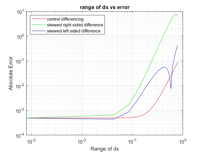
Result:

From the Graph, it is evident that Central Difference Scheme has very less error when compared with the Skewed Right Side Difference Scheme and Skewed Left Side Difference Scheme. So the value will more accurate in the Central Difference Scheme.