Week 3.5 - Deriving 4th order approximation of a 2nd order derivative using Taylor Table method
Aim :- Derive the following 4th order approximations of the second-order derivative.
Objective :- write a program in Matlab to evaluate the second-order derivative of the analytical function `e^x.cos(x)` and compare it with the 3 numerical approximations,
Central difference
Skewed right-sided differenc
Skewed left-sided difference
Theory/Calculations :-
Taylor's Series :
A Taylor Series is an expansion of some function into an infinite sum of terms, where each term has a larger exponent like x, x2, x3, etc.
Approximation :
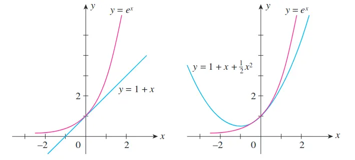
We can use the first few terms of a Taylor Series to get an approximate value for a function.
Here we can see example,where we can see the benifit of using approximation. Blue line is approximation.
Central Differencing:
We are going to derive the central differencing for the fourth order approximation of the second order derivative of a function using Taylor's table method.
In order to derive the central differencing we need to calculate the number of nodes or stencils required to evaluate the second order accurate.
For Central Differencing,
number of nodes, N = P+Q-1
where,
P = Order of the derivative.
Q = Order of Approximation.
For fourth order approximation of the second order derivative , the number of nodes required to derive central differencing is,
N = 2 + 4 - 1 = 5
The hypothesis of the second order derivative is expressed as,
`∇x^2f''(x)=af(i−2)+bf(i−1)+cf(i)+df(i+1)+ef(i+2)...........(1)`
Now evaluating each term of the hypothesis using taylor series,
`a f ( i − 2 ) = a [ f ( i ) − (2 ∇ x) /(1 !) f ' ( i ) + ( 2 ∇ x )^ 2 /(2 !) f ' ' ( i ) − ( 2 ∇ x )^ 3/( 3 !) f ' ' ' ( i ) + ( 2 ∇ x ) ^4 /(4 !) − ... ... ... ]`
`b f ( i − 1 ) = b [ f ( i ) − (∇ x) /(1 ! )f ' ( i ) + ( ∇ x ) ^2 /(2 !) f ' ' ( i ) − ( ∇ x )^ 3 /(3 !) f ' ' ' ( i ) + ( ∇ x ) ^4 /(4 !) − ... ... ... ]`
`c f ( i ) = c f ( i )`
`d f ( i + 1 ) = d [ f ( i ) + (∇ x )/(1 !) f ' ( i ) + ( ∇ x ) ^2/ (2 ! )f ' ' ( i ) + ( ∇ x ) ^3/( 3 !) f ' ' ' ( i ) + ( ∇ x ) ^4 /(4 !) − ... ... ... ]`
`e f ( i + 2 ) = e [ f ( i ) + (2 ∇ x) /(1 !) f ' ( i ) + ( 2 ∇ x )^ 2 /(2 !) f ' ' ( i ) + ( 2 ∇ x ) ^3 /(3 !) f ' ' ' ( i ) + ( 2 ∇ x ) ^4 /(4 ! )− ... ... ... ]`
Taylor's table for above equations,
| f(i)">f(i)f(i) | ∇xf′(i)">∇xf'(i)∇xf′(i) | ∇x2f′′(i)">∇x2f''(i)∇x2f′′(i) | ∇x3f′′′(i)">∇x3f'''(i)∇x3f′′′(i) | ∇x4f′′′′(x)">∇x4f''''(x)∇x4f′′′′(x) | |
| af(i-2)">af(i−2)af(i-2) | a | -2a | 4a/2 | -8a/6 | 16a/24 |
| bf(i-1)">bf(i−1)bf(i-1) | b | -b | b/2 | -b/6 | b/24 |
| cf(i)">cf(i)cf(i) | c | 0 | 0 | 0 | 0 |
| df(i+1)">df(i+1)df(i+1) | d | d | d/2 | d/6 | d/24 |
| ef(i+2)">ef(i+2)ef(i+2) | e | 2e | 4e/2 | 8e/6 | 16e/24 |
| Evaluation for 2nd order derivative | 0 | 0 | 1 | 0 | 0 |
With the help of the taylor's table we can find out the values of the coefficients by forming the equations,
`a + b + c + d + e = 0`
`− 2 a − b + d + 2 e = 0`
`4 a /2 + b /2 + d /2 + (4 e) /2 = 1`
`− (8 a) /6 − b /6 + d /6 + (8 e)/ 6 = 0`
`(16 a )/24 + b /24 + d /24 + (16 e)/ 24 = 0`
On solving the above equations we will get the values for coeffiecients and these coefficients value will then be put in equation 1 and hence the second order derivative for the fourth order approximation of the function for central differencing is evaluated.
Skewed right-sided difference:
In this case we are going to follow the same as procedure as we did in central differencing.
The number of nodes required,
N = P +Q
P = Order of the derivative.
Q = Order of Approximation.
For fourth order approximation of the second order derivative , the number of nodes required to derive skewed right-sided difference is,
N = 2 + 4 = 6.
The hypothesis of the second order derivative is expressed as,
`∇ x ^2 f ' ' ( x ) = a f ( i ) + b f ( i + 1 ) + c f ( i + 2 ) + d f ( i + 3 ) + e f ( i + 4 ) + g f ( i + 5 ) ... ... ... . . ( 2 )`
Now evaluating each term of the hypothesis using taylor series,
`a f ( i ) = a f ( i )`
`b f ( i + 1 ) = b [ f ( i ) + (∇ x) /(1 !) f ' ( i ) + ( ∇ x )^ 2/( 2 ! )f ' ' ( i ) + ( ∇ x )^ 3/( 3 !) f ' ' ' ( i ) + ( ∇ x ) ^4/( 4 !) − ... ... ... ]`
`c f ( i + 2 ) = c [ f ( i ) + (2 ∇ x)/( 1 !) f ' ( i ) + ( 2 ∇ x ) ^2/( 2 ! )f ' ' ( i ) + ( 2 ∇ x ) ^3/( 3 !) f ' ' ' ( i ) + ( 2 ∇ x )^ 4/( 4 ! )− ... ... ... ]`
`d f ( i + 3 ) = d [ f ( i ) + (3 ∇ x )/(1 !) f ' ( i ) + ( 3 ∇ x ) ^2 /(2 !) f ' ' ( i ) + ( 3 ∇ x ) ^3 /(3 !) f ' ' ' ( i ) + ( 3 ∇ x ) ^4 /(4 !) − ... ... ... ]`
`e f ( i + 4 ) = e [ f ( i ) + (4 ∇ x) /(1 !) f ' ( i ) + ( 4 ∇ x )^ 2/( 2 !) f ' ' ( i ) + ( 4 ∇ x )^ 3/( 3 !) f ' ' ' ( i ) + ( 4 ∇ x ) ^4/( 4 !) − ... ... ... ]`
`g f ( i + 5 ) = g [ f ( i ) +( 5 ∇ x) /(1 ! )f ' ( i ) + ( 5 ∇ x ) ^2 /(2 ! )f ' ' ( i ) + ( 5 ∇ x )^ 3 /(3 !) f ' ' ' ( i ) + ( 5 ∇ x )^ 4 /(4 ! )− ... ... ... ]`
Taylor's table for above equations,
| f(i)">f(i)f(i) | ∇xf′(i)">∇xf'(i)∇xf′(i) | ∇x2f′′(i)">∇x2f''(i)∇x2f′′(i) | ∇x3f′′′(i)">∇x3f'''(i)∇x3f′′′(i) | ∇x4f′′′′(x)">∇x4f''''(x)∇x4f′′′′(x) | ∇x5f′′′′′(x)">∇x5f'''''(x)∇x5f′′′′′(x) | |
| af(i)">af(i)af(i) | a | 0 | 0 | 0 | 0 | 0 |
| bf(i+1)">bf(i+1)bf(i+1) | b | b | b/2 | b/6 | b/24 | b/120 |
| cf(i+2)">cf(i+2)cf(i+2) | c | 2c | 4c/2 | 8c/6 | 16c/24 | 32c/120 |
| df(i+3)">df(i+3)df(i+3) | d | 3d | 9d/2 | 27d/6 | 81d/24 | 243d/120 |
| ef(i+4)">ef(i+4)ef(i+4) | e | 4e | 16e/2 | 64e/6 | 256e/24 | 1024e/120 |
| gf(i+5)">gf(i+5)gf(i+5) | g | 5g | 25g/2 | 125g/6 | 625g/24 | 3125g/120 |
| Evaluation for 2nd order derivative | 0 | 0 | 1 | 0 | 0 | 0 |
With the help of the taylor's table we can find out the values of the coefficients by forming
`a + b + c + d + e + g = 0`
`b + 2 c + 3 d + 4 e + 5 g = 0`
`b/ 2 + (4 c)/ 2 + (9 d )/2 + (16 e )/2 + (25 g)/ 2 = 1`
`b /6 + (8 c)/ 6 + (27 d )/6 + (64 e) /6 + (125 g)/ 6 = 0`
`b /24 + (16 c )/24 + (81 d)/ 24 + (256 e) /24 + (625 g )/24 = 0`
`b /120 + (32 c )/120 + (243 d) /120 + (1024 e) /120 + (3125 g) /120 = 0`
On solving the above equations we will get the values for coeffiecients and these coefficients value will then be put in equation 2 and hence the second order derivative for the fourth order approximation of the function for right-sided differencing is evaluated.
Skewed left-sided difference:
In this case we are going to follow the same as procedure as we did in right - sided differencing.
The number of nodes required,
N = P+Q
P = Order of the derivative.
Q = Order of Approximation.
For fourth order approximation of the second order derivative , the number of nodes required to derive skewed right-sided difference is,
N = 2 + 4 = 6.
The hypothesis of the second order derivative is expressed as,
`∇ x ^2 f ' ' ( x ) = a f ( i − 5 ) + b f ( i − 4 ) + c f ( i − 3 ) + d f ( i − 2 ) + e f ( i − 1 ) + g f ( i ) ... ... ... . . ( 3 )`
Now evaluating each term of the hypothesis using taylor series,
`a f ( i − 5 ) = a [ f ( i ) − (5 ∇ x) /(1 !) f ' ( i ) + ( 5 ∇ x ) ^2 /(2 ! )f ' ' ( i ) − ( 5 ∇ x ) ^3 /(3 !) f ' ' ' ( i ) + ( 5 ∇ x ) ^4 /(4 !) − ... ... ... ]`
`b f ( i − 4 ) = b [ f ( i ) − (4 ∇ x )/(1 !) f ' ( i ) + ( 4 ∇ x ) 2 /(2 ! )f ' ' ( i ) − ( 4 ∇ x ) 3 /(3 ! )f ' ' ' ( i ) + ( 4 ∇ x ) 4 /(4 ! )− ... ... ... ]`
`c f ( i − 3 ) = c [ f ( i ) − (3 ∇ x) /(1 !) f ' ( i ) + ( 3 ∇ x ) ^2 /(2 !) f ' ' ( i ) − ( 3 ∇ x ) ^3/( 3 !) f ' ' ' ( i ) + ( 3 ∇ x )^ 4 /(4 ! )− ... ... ... ]`
`d f ( i − 2 ) = d [ f ( i ) − (2 ∇ x) /(1 !) f ' ( i ) + ( 2 ∇ x )^ 2 /(2 !) f ' ' ( i ) − ( 2 ∇ x )^ 3 /(3 ! )f ' ' ' ( i ) + ( 2 ∇ x ) ^4/( 4 ! )− ... ... ... ]`
`e f ( i − 1 ) = e [ f ( i ) − (∇ x)/ (1 !) f ' ( i ) + ( ∇ x ) ^2 /(2 !) f ' ' ( i ) − ( ∇ x ) ^3/ (3 !) f ' ' ' ( i ) + ( ∇ x ) ^4 /(4 ! )− ... ... ... ]`
`g f ( i ) = g f ( i )`
Taylor's table for above equations,
| f(i)f(i) | ∇xf'(i)∇xf′(i) | ∇x2f''(i)∇x2f′′(i) | ∇x3f'''(i)∇x3f′′′(i) | ∇x4f''''(x)∇x4f′′′′(x) | ∇x5f'''''(x)∇x5f′′′′′(x) | |
| af(i−5)af(i-5) | a | -5a | 25a/2 | -125a/6 | 625a/24 | -3125a/120 |
| bf(i−4)bf(i-4) | b | -4b | 16b/2 | -64b/6 | 256b/24 | -1024b/120 |
| cf(i−3)cf(i-3) | c | -3c | 9c/2 | -27c/6 | 81c/24 | -243c/120 |
| df(i−2)df(i-2) | d | -2d | 4d/2 | -8d/6 | 16d/24 | -32d/120 |
| ef(i−1)ef(i-1) | e | -e | e/2 | -e/6 | e/24 | -e/120 |
| gf(i)gf(i) | g | 0 | 0 | 0 | 0 | 0 |
| Evaluation for 2nd order derivative | 0 | 0 | 1 | 0 | 0 | 0 |
With the help of the taylor's table we can find out the values of the coefficients by forming the equations,
`a + b + c + d + e + g = 0`
`− 5 a − 4 b − 3 c − 2 d − e = 0`
`(25 a) /2 + (16 b)/ 2 + (9 c) /2 +( 4 d )/2 + e/ 2 = 1`
`(− 125 a) /6 + (− 64 b)/ 6 +( − 27 c)/ 6 + (− 8 d) /6 + (− e) /6 = 0`
`(625 a) /24 + (256 b) /24 + (81 c) /24 + (16 d )/24 + e /24 = 0`
`(− 3125 a) /120 + (− 1024 b )/120 +( − 243 c)/ 120 + (− 32 d) /120 + − e /120 = 0`
On solving the above equations we will get the values for coeffiecients and these coefficients value will then be put in equation 3 and hence the second order derivative for the fourth order approximation of the function for left-sided differencing is evaluated.
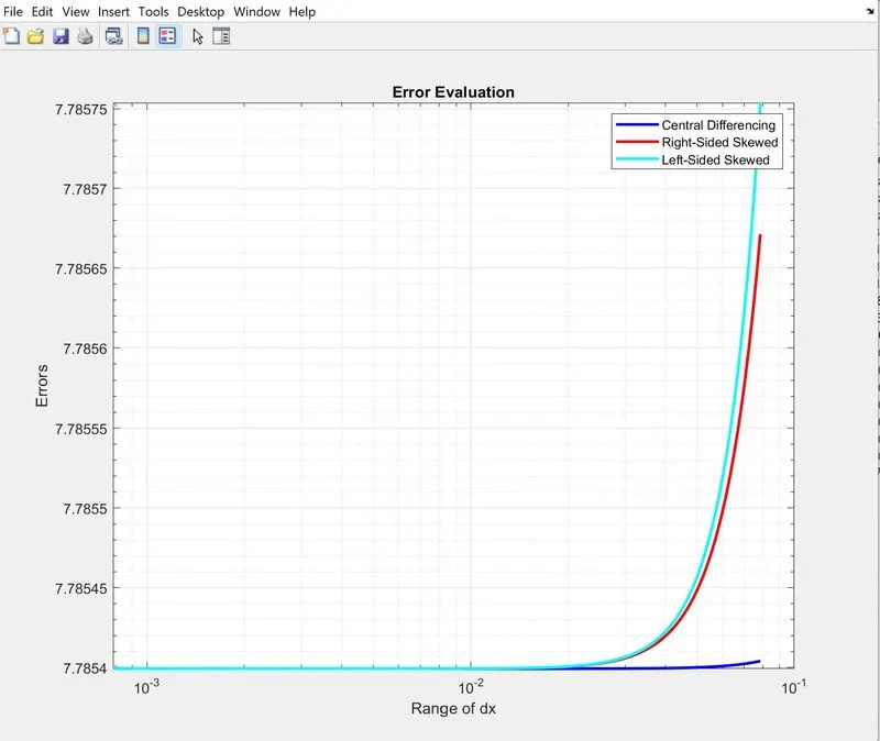
Now that we have derived all the equations for second order derivative using Central differencing, Right-sided difference and Left-sided difference schemes, we are going to evaluate it using MATLAB program and plotting the results showing the absolute errors with ranges of dx.
Why Skewed ??
The skewed scheme is useful because it is necessary to compute the grids at the corners also which central differecing scheme is unable to do. Symmetric nodes does not present on the corners so that CD can not be implemented in such conditions.
Matlab Code :-
clear all
close all
clc

%Using taylor table method we are going to find out the second order
%derivative for fourth order approximation
% Function, f(x) = exp(x).cos(x)
x = pi/3;
dx = linspace(pi/4000,pi/40,100);
% Calculating the second order analytical derivative of the function
analytical_derivative = -2*exp(x)*sin(x);

% Central Differencing
a_central = [1 1 1 1 1;-2 -1 0 1 2;4/2 1/2 0 1/2 4/2;-8/6 -1/6 0 1/6 8/6;16/24 1/24 0 1/24 16/24];

b_central = [0;0;1;0;0];

c_central = inv(a_central) * b_central;

% Calculating second order numerical derivative using Central differencing
central_differencing = (c_central(1)*(exp(x-dx*2).*sin(x-dx*2)) + c_central(2)*(exp(x-dx).*sin(x-dx)) + c_central(3)*(exp(x).*sin(x)) + c_central(4).*(exp(x+dx).*sin(x+dx)) + c_central(5).*(exp(x+dx*2).*sin(x+dx*2)))./(dx.^2);

% Absolute error between second order derivative of analytical and central
% differencing scheme
central_error = abs(central_differencing - analytical_derivative);

%Right Sided Skewed
a_right  = [1 1 1 1 1 1;0 1 2 3 4 5;0 1/2 4/2 9/2 16/2 25/2;0 1/6 8/6 27/6 64/6 125/6;0 1/24 16/24 81/24 256/24 625/24;0 1/120 32/120 243/120 1024/120 3125/120];

b_right = [0;0;1;0;0;0];

c_right = inv(a_right) * b_right;

% Calculating second order numerical derivative using Central differencing
skewed_right = (c_right(1).*(exp(x)*sin(x)) + c_right(2).*(exp(x+dx).*sin(x+dx)) + c_right(3).*(exp(x+2*dx).*sin(x+2*dx)) + c_right(4).*(exp(x+3*dx).*sin(x+3*dx)) + c_right(5).*(exp(x+4*dx).*sin(x+4*dx)) + c_right(6).*(exp(x+5*dx).*sin(x+5*dx)))./(dx.^2);

% Absolute error between second order derivative of analytical and skewed right-sided scheme
skewed_right_error = abs(skewed_right - analytical_derivative);

% Left Sided Skewed
a_left  = [1 1 1 1 1 1;-5 -4 -3 -2 -1 0;25/2 16/2 9/2 4/2 1/2 0;-125/6 -64/6 -27/6 -8/6 -1/6 0;625/24 256/24 81/24 16/24 1/24 0;-3125/120 -1024/120 -243/120 -32/120 -1/120 0];

b_left = [0;0;1;0;0;0];

c_left = inv(a_left) * b_left;

% Calculating second order numerical derivative using Central differencing
skewed_left = (c_left(1).*(exp(x-5*dx).*sin(x-5*dx)) + c_left(2).*(exp(x-4*dx).*sin(x-4*dx)) + c_left(3).*(exp(x-3*dx).*sin(x-3*dx)) + c_left(4).*(exp(x-2*dx).*sin(x-2*dx)) + c_left(5).*(exp(x-dx).*sin(x-dx)) + c_left(6).*(exp(x)*sin(x)))./(dx.^2);

% Absolute error between second order derivative of analytical and skewed left-sided scheme
skewed_left_error = abs(skewed_left - analytical_derivative);

% Plotting the results
loglog(dx,central_error,'color','b','linewidth',2);
hold on
loglog(dx,skewed_right_error,'color','r','linewidth',2);
hold on
loglog(dx,skewed_left_error,'color','c','linewidth',2);
grid on
legend('Central Differencing','Right-Sided Skewed','Left-Sided Skewed')
xlabel('Range of dx')
ylabel('Errors')
title('Error Evaluation')
Output :-