Week 3 - Solving second order ODEs

Aim :- To solve second order ODE using matlab.

Objective :- Solving a second order ode using matlab to see motion of a simple pendulum and create a frames that can generate animation of pendulum oscillation.

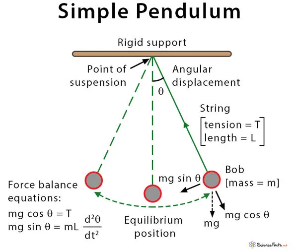
Theory :- Simple pendulum have two points one is fixed and another is free.Mass(m) is attach to the free end to move the pendulum along its axis.With the help of the string fixed point and free point are join together to generate a simple harmonic motion.

Simple Harmonic Motion :- Simple Harmonic Motion or SHM is a specific type of oscillation in which the restoring force is directly proportional to the displacement of the particle from the mean position.

Mean Position :- The position at which the net force on the particle in SHM is zero is known as the mean position.

Extreme position :- The Position located at the distance equal to the amplitude of the SHM is known as extreme position.

Time Period :- The time interval after which the particle comes in same phase.Time period is given by

T = 2π √g/√l

Calculations :-

Required Parameters(Assume),

b = damping coefficient

= 0.05

g = gravity

= 9.81 m/s^2

l = length of the pendulum in m

= 1 m

m = mass of the ball in kg

= 1 kg

Given parameters,

time = 0 to 20sec (simulation time)

angular displacement = 0

angular velocity = 3rad/sec

Applying newton's second law of rotational motion we can able to calculate motion of the pendulum with damping coefficient.

(d^2_theta/dt^2) + (d_theta/dt)*(b/m) + g/l.*sin(theta) = 0

theta = theta1(assume)

d_theta/dt = d_theta1/dt

d_theta1/dt = theta2 -eq(1)

d^2_theta1/dt^2 = d/dt(d_theta1/dt) = d/dt(theta2)

d_theta2/dt = -b/m(theta2) - g/m.*sin(theta1)

Breaking down equation in matrix form

d/dt [theta1 ; theta2] = [theta2 ; -b/m(theta2) - g/m.*sin(theta1)]

Note : I tried to write down above equation with the help of the math symbols but it isn't working.

Code :-

Code below shows the plot that contains angular displacement and angular velocity.

close all
clear all
clc

% second order ordinary diffential equation (ODE)

% Inputs
b = 0.05;
g = 9.81;
l = 1;
m = 1;

% Initial condition
theta_0 = [0;3];

%time points
t_span = linspace(0,20,300);

% solve ode
[t,results] = ode45(@(t,theta) ode_function(t,theta,b,g,l,m),t_span,theta_0);

figure(1)
plot(t,results(:,1))
hold on
plot(t,results(:,2))
title('second order ode')
xlabel('t')
ylabel('theta')
legend('angular disp','angular value')
grid on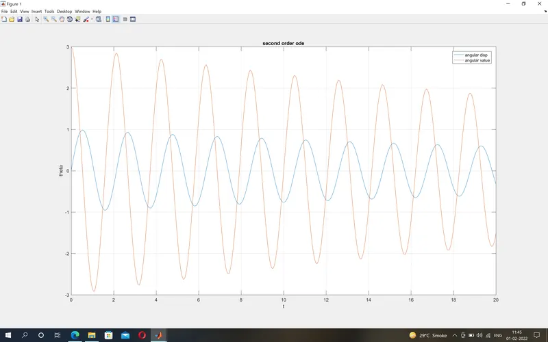

In the above code we use function 'ode45'.We define that function seperately to use in this code and it also makes convinient for us to use in our main code.ode45 is also a solver available in a matlab.

Function,

[t,results] = ode45(@(t,theta) ode_function(t,theta,b,g,l,m),t_span,theta_0)

Input arguments of the above function we define it earlier in the code.

Code = ode_function

function [dtheta_dt] = ode_function(t,theta,b,g,l,m)

   theta1 = theta(1)
   theta2 = theta(2)
   dtheta1_dt = theta2;
   dtheta2_dt = -(b/m)*theta2 - (g/l)*sin(theta1);
   dtheta_dt = [dtheta1_dt;dtheta2_dt];
end

To create a animation of the simple pendulum we need to extend our code and introduced for loop in it.In for loop we need to provide co-ordinates values that gives us string oscillation.

Main code :-

close all
clear all
clc

% second order ordinary diffential equation (ODE)

% Inputs
b = 0.05;
g = 9.81;
l = 1;
m = 1;

% Initial condition
theta_0 = [0;3];

%time points
t_span = linspace(0,20,300);

% solve ode
[t,results] = ode45(@(t,theta) ode_function(t,theta,b,g,l,m),t_span,theta_0);

% first plot that shows time vs theta plot
figure(1)
plot(t,results(:,1))
hold on
plot(t,results(:,2))
title('second order ode')
xlabel('t')
ylabel('theta')
legend('angular disp','angular value')
hold off
grid on

  % to create a movie
displacement = results(:,1);
velocity = results(:,2);
  
x0 = 1;
y0 = 1;
ct = 1;
  for i = 1:length(displacement)
     
      x1 = 1-l*sin(displacement(i));
      y1 = 1-l*cos(displacement(i));
      
    figure(2)
       
      plot([0 2],[1 1],'linewidth',5,'color','b');
      hold on
      % plot coordinates with color and its diamensions
      plot([1,x1],[1 y1],[x1 x1],[y1 y1],'-o','markersize',25,'markerfacecolor','r','linewidth',4);
      axis([0 2 -0.5 2])
      
      %to capture current figure
      M(ct) = getframe(gcf);
      %loop counter
      ct = ct+1;
      hold off
      
  end
  
  % to create a video file of the generated frames we need to use array  
  movie(M)
  videofile = VideoWriter('simple_pendulum.avi','uncompressed AVI');
  open(videofile)
  writeVideo(videofile,M)
  close(videofile)

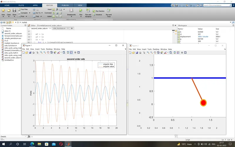
At the end of the programe we use movie(M) array to get the movie of the generated frames.Format of the movie is AVI.

Output :-

Google photos link to watch Simple Pendulim Oscillation :-

https://photos.app.goo.gl/DwDVjtzrXDgivU3TA

Conclusion :- Here we can conclude that using matlab we get angular displacement and angular veocity graph,and also we are able to see oscillation of the simple pendulum with various theta position at a different time interval.