Week 4.1 - Genetic Algorithm

Aim :- To solve global optimization problem using and understanding genetic algorithm in matlab.Also find global maxima of the given function.

Objective :- Mainly understanding how GA works and defining stalagmite function for maxima for finding global maxima.

Theory :-

Optimization :- The main goal of process optimization is to reduce or eliminate time and resource wastage, unnecessary costs,and mistakes while achieving the process objective. We only spend time correcting an error if the mistake exists.A specific optimization problem involves minimizing or maximizing systematically by choosing input values within an allotted set and finding the function’s value. It applies a large area of mathematics for generalizing theory of optimization. Optimization involves determining best available values of the particular objective function in a define domain along with a variety of different types of objective functions.

Genetic algorithm is also one of the optimization process.

Genetic Algorithm (GA) :- The genetic algorithm is a method for solving both constrained and unconstrained optimization problems that is based on natural selection, the process that drives biological evolution. The genetic algorithm repeatedly modifies a population of individual solutions. At each step, the genetic algorithm selects individuals at random from the current population to be parents and uses them to produce the children for the next generation. Over successive generations, the population "evolves" toward an optimal solution.

"GA always minimizes the function".

GA always uses some rules to create a next generation population

Fitness Function :- The fitness function is simply described as a function that takes as input a potential solution to a problem and gives as output how “fit” or how “excellent” the answer is in relation to the problem under discussion.

Selection :- It selects the individuals called parents that contribute to the population for the next generation,which are more fit they are usually selected

Crossover :- It combines two parents to form children for the next generation,it helps to create more population.

Mutation :- It applies random changes to individual parents to form children for the next sampling or generation.

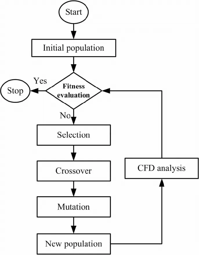
Above flow chart shows how optimizaton process works.

Stalagmite Function :-

Using given equation we need to create a function that we have to use in the optimization problem.

Eq :- f(x,y) = f1,fx2,xf1,yf2,y

f(x1) = (sin(5.1*pi*x + 0.5))^6

f(y1) = (sin(5.1*pi*y + 0.5))^6

f(x2) = exp(-4*log(2)*((x-0.0667^2)/0.64))

f(y2) = exp(-4*log(2)*((y-0.0667^2)/0.64)).

Code (stalagmite function) :-

function [V] = stalagmite_f(input)
    x = input(1); % variable 1
    y = input(2); % variable 2
    
    x1 = (sin(5.1*pi*x+0.5))^6;
    y1 = (sin(5.1*pi*y+0.5))^6;
    x2 = exp(-4*log(2)*((x-0.0667)^2)/0.64);
    y2 = exp(-4*log(2)*((y-0.0667)^2)/0.64);
    
    V = x1*y1*x2*y2*-1 
end

Stalagmite function help us to find local maxima and minima.We know that GA always find global minima for the given function,so we need to modify our function so GA will gives us global maxima.So we introduce '-' minus sign in the function so the output will be the global maxima.

Matlab Case Study :-

In this study we just introducing our stalagmite function without any constraints,to see how it behave.

Here we are using two variables x and y as given in the equation,and also using linspace command and num case which is iteration number. Given x and y are one diamensional hence we are using mesh grid command to create two diamensional array which represents xx and yy.

Here we are using for loop also,this for loop will run for the length of xx and yy. It is a roe vector and it has two column which are assign using input(1) and input(2).Our main intention from the for loop is that to create a three diamensional graph to make it easy to understand.

Code (With loop and function) :-

close all
clear all
clc

% writing a code to generate a genetic algorithm
% defining search space 
x = linspace(0,0.6,150);
y = linspace(0,0.6,150);
num_case = 50;

% generating 2d mesh
[xx,yy] = meshgrid(x,y);

% using stalagmite function

for i = 1:length(xx)
    for j = 1:length(yy)
        input(1) = xx(i,j);
        input(2) = yy(i,j);
      f(i,j) = stalagmite_f(input);
    end
end

surfc(xx,yy,f)
shading interp

Output :-

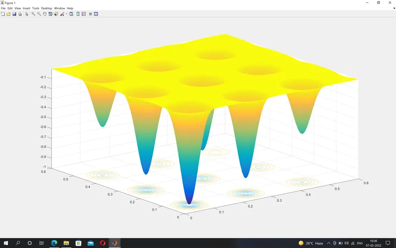
Matlab case study 1:-

Case study with no bounds.

The syntax we are using here is,[coordinates,fopt(i)] = ga(@stalagmite,2).

Here after @ sign we are using function i.e., Stalagmite.

Number of variables are 2 thats why we are using 2 after function.

Here we are using for loop for 50 cases.

To get optimize result of the given eq we are running genetic algorithm function to optimize the stalagmite function as input.This will gives optimize results.

The new values we are getting with optimization it getting stored in the variable called xopt,yopt and fopt respectively.

Time taken for optimization being calculated using tic and toc command.

To plot 3d graph we use optimized values.

Code study 1:-

close all
clear all
clc

% writing a code to generate a genetic algorithm
% defining search space 
x = linspace(0,0.6,150);
y = linspace(0,0.6,150);
num_case = 50;
[xx,yy] = meshgrid(x,y);

% using stalagmite function

for i = 1:length(xx)
    for j = 1:length(yy)
        input(1) = xx(i,j);
        input(2) = yy(i,j);
      f(i,j) = stalagmite(input);
    end
end
surfc(xx,yy,f)

tic
for i = 1:num_case
    [coordinates,fopt(i)] = ga(@stalagmite,2);
    xopt(i) = coordinates(1);
    yopt(i) = coordinates(2);
end

% To calculate time required for study1
 study1_time = toc
 figure(1)
 subplot(2,1,1)
 hold on
 surf(xx,yy,-f)
 shading interp
 xlabel('xx')
 ylabel('yy')
 zlabel('f')
 hold on
 plot3(xopt,yopt,-fopt,'marker','o','markersize',6)
 title('unbounded coordinates')
 subplot(2,1,2)
 plot(fopt)
 xlabel('iteration')
 ylabel('function maxima')

Output :-

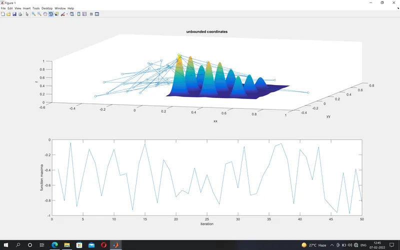
Time taken for study 1 is = 5.2064sec.

Case Study 2 :-

Here we are using upper and lower bounds for the GA.

Syntax we are using here is [coordinates,fopt(i)] = ga(@stalagmite,2,[],[],[],[],[0;0],[1;1]).

In the above syntax first we use function i.e, stalagmite.

After function number of variables is written i.e, 2.

([],[]) ,1st 2 empty square bracket shows linear inequalities in the form of A*x<=B.

([],[]),Number 3 and 4 empty brackets shows linear equalities of the form A*x=B.

And last two filled square brackets shows lower and upper bounds in which GA will search results.

Code study 2:-

close all
clear all
clc

% writing a code to generate a genetic algorithm
% defining search space 
x = linspace(0,0.6,150);
y = linspace(0,0.6,150);
num_case = 50;
[xx,yy] = meshgrid(x,y);

% using stalagmite function

for i = 1:length(xx)
    for j = 1:length(yy)
        input(1) = xx(i,j);
        input(2) = yy(i,j);
      f(i,j) = stalagmite(input);
    end
end
surfc(xx,yy,f)

tic
for i = 1:num_case
    [coordinates,fopt(i)] = ga(@stalagmite,2,[],[],[],[],[0;0],[1,1]);
    xopt(i) = coordinates(1);
    yopt(i) = coordinates(2);
end

% To calculate time required for study1
 study2_time = toc
 figure(1)
 subplot(2,1,1)
 hold on
 surf(xx,yy,-f)
 shading interp
 xlabel('xx')
 ylabel('yy')
 zlabel('f')
 hold on
 plot3(xopt,yopt,-fopt,'marker','o','markersize',6)
 title('Bounded Inputs')
 subplot(2,1,2)
 plot(fopt)
 xlabel('iteration')
 ylabel('function maxima')

Output :-

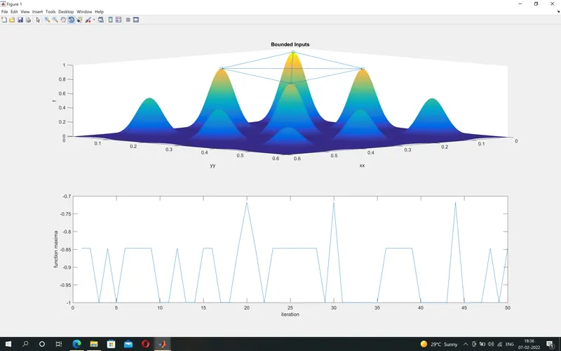
Time taken for study 2 is 5.5849sec.Here as u can see time for study 2 is slightly bigger than study 1.

Case study 3 :- In this case study we are going to increase the population size from 150 to 450.Increasing number of iteration gives us optimum function value.While increasing the population size keep in mind that increasing value in bigger amount will slow down the GA.

Syntax,

([],[]),After upper and lower boundaries we are adding to more empty square brackets it denotes no non linear constraints exists.

(Options),To provide value of the population.

Syntax for study 3,[coordinates,fopt(i)] = ga(@stalagmite,2,[],[],[],[],[0;0],[1;1],[],[],options).

Code Case Study 3 :-

close all
clear all
clc

% writing a code to generate a genetic algorithm
% defining search space 
x = linspace(0,0.6,150);
y = linspace(0,0.6,150);
num_case = 50;
[xx,yy] = meshgrid(x,y);

% using stalagmite function

for i = 1:length(xx)
    for j = 1:length(yy)
        input(1) = xx(i,j);
        input(2) = yy(i,j);
      f(i,j) = stalagmite(input);
    end
end

% To increase GA iteration
options = optimoptions('ga')
options = optimoptions(options,'populationSize',450);

tic
for i = 1:num_case
    [coordinates,fopt(i)] = ga(@stalagmite,2,[],[],[],[],[0;0],[1,1],[],[],options);
    xopt(i) = coordinates(1);
    yopt(i) = coordinates(2);
end

% To calculate time required for study3
 study3_time = toc
 figure(1)
 subplot(2,1,1)
 hold on
 surf(xx,yy,-f)
 shading interp
 xlabel('xx')
 ylabel('yy')
 zlabel('f')
 hold on
 plot3(xopt,yopt,-fopt,'marker','*','markersize',9)
 title('Bounded Inputs')
 subplot(2,1,2)
 plot(fopt)
 xlabel('iteration')
 ylabel('function maxima')

Output Case Study 3 :-

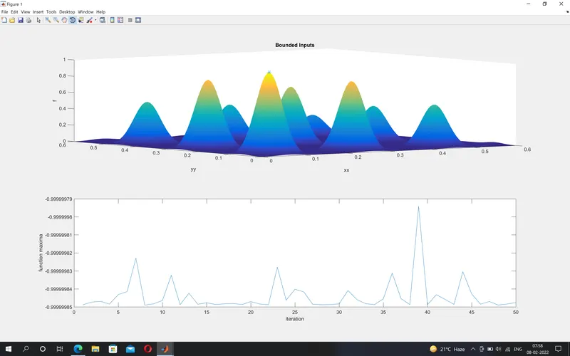
Time taken by study 3 is 25.0986sec ,which is much bigger than our previous studies.

In the above graph you can see that GA has found the global maxima.(*) shows the global maxima.

Conclusion :- In this Challenge we learn how to find global maxima instead of global minima,with increasing population size.Also how to use function in the GA.