Week 3.5 - Deriving 4th order approximation of a 2nd order derivative using Taylor Table method

A Taylor series is a series expansion of a function about a point. It represents a function as a infinite sum of derivatives. one dimensional Taylor series for a function at X=a is given by,

F(x)=f(a)+f’a*(x-a)+f’’(a)/2! (x-a)²+f’’’(a)/2!(x-a)³+…….fⁿ(a)/n!(x-a)ⁿ

If the value of a=0, then the series is Maclaurin series.

Solution for Central difference schemes

Number of nodes = P+Q-1 = 2+4-1 = 5

For 4^th order approximation, 5 points stencil points are taken as below.

……………….*……………….*………………..*…………………….*………………………..*………………..

(i-2) (i-1) (i) (i+1) (i+2)

2^nd order derivative is as below.

d²u/dx²=[af(i-2)+bf(i-1)+cf(i)+df(i+1)+ef(i+2)]/dx²………..(1)

To obtain 4^th order approximation, for the above eqiuation(1)

af(i-2)=af(i)-{[2af’(i)dx]/1!}+{[4af’’(i)dx²]/2!}+{[8af’’’(i)dx³]/3!}+{[16af’’’’(i)dx⁴]/4!}

Similarly for all other points been expressed and tabulated as below.

Above table is been solved on matrix inversion method.

1 1 1 1 1 a 0

-2 -1 0 1 2 b 0

2 ½ 0 ½ 2 * c = 1

-4/3 -1/6 0 1/6 4/3 d 0

2/3 1/24 0 1/24 2/3 e 0

X=inv(A)*B

Solution:

a = -0.0833

b = 1.3333

c = -2.5

d = 1.3333

e = -0.0833

Substituting these values in equation (1)

d²u/dx²=[-0.0833f(i-2)+1.3333f(i-1)+(-2.5)f(i)+1.3333f(i+1)+(-0.0833)f(i+2)]/dx²

Solution for right difference schemes

Number of nodes = P+Q = 2+4 = 6

For 4^th order approximation, 5 points stencil points are taken as below.

……………….*……………….*………………..*…………………….*………………………..*………………..*……………….

(i) (i+1) (i+2) (i+3) (i+4) (i+5)

2^nd order derivative is as below.

d²u/dx²=[af(i)+bf(i+1)+cf(i+2)+df(i+3)+ef(i+4) +gf(i+5) ]/dx²………..(2)

Above table is been solved on matrix inversion method.

1 1 1 1 1 1 a 0

0 1 2 3 4 5 b 0

0 ½ 4/2 9/2 16/2 25/2 * c = 1

0 1/6 8/6 27/6 64/6 125/6 d 0

0 1/24 16/24 81/24 256/24 625/24 e 0

0 1/120 32/120 243/120 1024/120 3125/120 g 0

X=inv(A)*B

Solution:

a = 3.7500

b = -12.8333

c = 17.8333

d = -13.000

e = 5.0833

g = -0.8333

Substituting these values in equation (2)

d²u/dx²=[3.75f(i)+(-12.8333)f(i+1)+17.8333f(i+2)+(-13.000)f(i+3)+5.0833f(i+4) +(-0.8333)f(i+5) ]/dx²

Solution for left difference schemes

Number of nodes = P+Q = 2+4 = 6

For 4^th order approximation, 5 points stencil points are taken as below.

……………….*……………….*………………..*…………………….*………………………..*………………..*……………….

(i-5) (i-4) (i-3) (i-2) (i-1) (i)

2^nd order derivative is as below.

d²u/dx²=[af(i-5)+bf(i-4)+cf(i-3)+df(i-2)+ef(i-1) +gf(i) ]/dx²………..(3)

X=inv(A)*B

Solution:

a = -0.8333

b = 5.0833

c = -13.0000

d = 17.8333

e = -12.8333

g = 3.7500

Substituting these values in equation (3)

d²u/dx²=[(-0.8333)f(i-5)+5.0833f(i-4)+(-13.000)f(i-3)+17.833f(i-2)+(-12.8333)f(i-1) +3.7500f(i) ]/dx²

clear all
close all
clc

x=pi/3;

dx = linspace(pi/4, pi/4000,40);

for i=1:length(dx)
central_differencing(i)=fourth_order_central_differencing(x,dx(i));
right_skew_differencing(i)=fourth_order_right_skew(x,dx(i));
left_skew_differencing(i)=fourth_order_left_skew(x,dx(i));
end

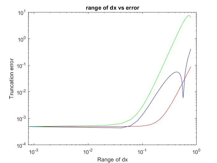
figure(1)
loglog(dx,central_differencing,'r')
hold on
loglog(dx,right_skew_differencing,'g')
hold on
loglog(dx,left_skew_differencing,'b')
xlabel('Range of dx')
ylabel('Truncation error')
title('range of dx vs error')

function error_right_skew = fourth_order_right_skew(x,dx);
analytical_derivative = -2*exp(x)*sin(x);
right_skew_differencing = ((((3.750)*((exp(x))*(cos(x))))-((12.8333)*((exp(x+dx))*(cos(x+dx))))+((17.8333)*((exp(x+(2*dx)))*(cos(x+2*dx))))-((13.000)*((exp(x+3*dx)))*(cos(x+3*dx))))+((5.0833)*((exp(x+4*dx)))*(cos(x+(4*dx))))-(0.8333)*((exp(x+(5*dx)))*(cos(x+(5*dx)))))/(dx^2);
error_right_skew = abs(right_skew_differencing - analytical_derivative);
end

Solution:

Central difference scheme is better than other 2 schemes with less errors.
Plotted results shows the same.