Week 9 - FVM Literature Review

Aim:- Explain the major differences between FDM & FVM and understand the need for interpolation schemes and flux limiters in FVM.

Theory: In Fluid Dynamics there are three numerical-method-based solvers which are used to solve for the governing equation of Navier-Stokes

- Finite Difference Method

- Finite Element Method

- Finite Volume Method

Finite Volume Method(FVM) -

The Finite Volume Method (FVM) is a discretization method for the approximation of a single or a system of partial differential equations expressing the conservation, or balance, of one or more quantities. These partial differential equations (PDEs) are often called conservation laws; they may be of different nature, e.g. elliptic, parabolic or hyperbolic. They describe the relations between partial derivatives of unknown fields such as temperature, concentration, pressure, with respect to variables within the domain (space, time,...) under consideration.

As in the finite element method, a mesh is constructed, which consists of a partition of the domain where the space variable lives. The elements of the mesh are called control volumes. The integration of the PDE over each control volume results in a balanced equation. The set of balance equations is then discretized with respect to a set of discrete unknowns. The main issue is the discretization of the fluxes at the boundaries of each control volume: in order for the FVM to be efficient, the numerical fluxes are generally

conservative, i.e. the flux entering a control volume from its neighbor must be the opposite of the one entering the neighbor from the control volume,
consistent, i.e. the numerical flux of a regular function interpolation tends to the continuous flux as the mesh size vanishes.

It is sometimes possible to discretize the fluxes at the boundaries of the control volume by the finite difference method (FDM). In this case, the method has often been referred to as a finite difference method or conservative finite difference method. The specificity of the FVM with respect to the FDM is that the discretization is performed on the local balance equations, rather than the PDE: the fluxes on boundaries of the control volumes are discretized, rather than the continuous differential operator.

The resulting system of discrete equations depends on a discrete (finite) set of unknowns, and may be either linear or non-linear, depending on the original problem itself; this system is then solved exactly or approximately, using for example direct or iterative solvers in the case of linear equations and fixed point or Newton-type methods in the case of nonlinear equations.

Differences between Finite Difference Method (FDM) and Finite Volume Method (FVM)

Finite Difference Method (FDM):

- A Finite Difference Method discretization is based upon the differential form of governing equation to be solved

- FDM describes an unknown variable Ï• by means of point samples at node points. Truncated Taylor series expansions are used to generate finite difference approximations to the derivatives of Ï• at each grid point and its immediate neighbors.

- It is important in FDM that the meshing is structured/aligned grids for which each node governing equations are solved.

- Advantages: Ease of implementation.

- Disadvantages: Restricted to simple grids and does not conserve momentum, energy, and mass on coarse grids.

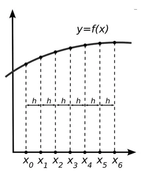
Example- In order to calculate the solution for the entire domain, first we discretize it into small elements and nodal coordinates are generated. The governing equations are solved for each and every node iteratively until the expected convergence is achieved.

Let us take an example of 1D steady-state heat conduction

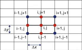
To calculate for a particular point.

Let's calculate for Temperature(T), using the meshing points using the second-order central differencing scheme,

`(del^2T)/(del x^2)= (T_(i-1,j) - 2T_(i,j) + T_(i+1,j))/(Deltax^2)`

The above equation represents the Finite-Difference discretization approach calculated at the nodal coordinates (grid points) of a domain.

Finite Volume Method (FVM):

- A Finite Volume Method discretization is based upon the integral form of the governing equation to be solved.

- The PDE is written to solve for a given finite volume. The computational domain is discretized into finite volumes and then for every volume governing equations are solved.

- The resulting system of equations usually involves the fluxes of a conserved variable and thus the calculation of fluxes is very important in FVM.

- The FVM is popular in fluid mechanics because it rigorously enforces conservation and it is flexible in terms of both geometry and the variety of fluid.

- Advantages:
- Basic FV control volume balance does not limit cell shape; mass, momentum, energy conserved even on coarse grids; efficient, iterative solvers well developed.

- FVM is flexible to deal with unstructured grids and can be applied to complex geometries and moving parts.

- Disadvantages: False diffusion when simple numerics are used.

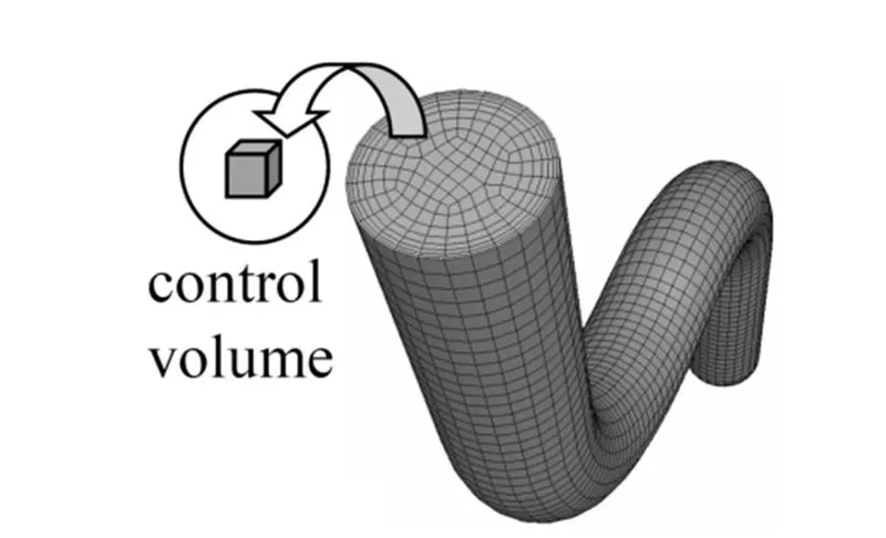
Example- The domain is divided into small chunks of control volume (discretized boxes or in case of any arbitrary shape). These control volumes have a center point (centroid) representing the control volume as (i-1), (i), and (i+1).

Figure- Cell-centered finite volume 2D grid. A node at the center of each cell represents the location where terrain elevations and tillage directions are given, and the control volume boundary is nothing but the face between the adjacent control volume.

- The vertical dividing line between control volumes is nothing but the face from which flux of a conserved variable will be taken into account.

- The governing equations of PDE are solved for a control volume and then integrated to calculate for the whole domain.

How does FVM solve the problem-

- In FVM, we write the equation of a volume instead of writing it for a point, which means inside a volume(of any shape) we assume the flow is conserved, the flow quantities(energy, mass, momentum) are conserved, this is called FVM representation.

- Then we apply the mathematical techniques to solve governing equations for the entire control volume.

Finite volume methods can be compared and contrasted with the finite difference methods, which approximate derivatives using nodal values, or finite element methods, which create local approximations of a solution using local data, and construct a global approximation by stitching them together. In contrast, a finite volume method evaluates exact expressions for the average value of the solution over some volume and uses this data to construct approximations of the solution within cells

Steps to discretize in Finite Volume

- Writing the governing equations in their integral form, as we take infinitesimal control volume and apply governing equation of the partial differential form. In order to calculate it for whole control volume (domain), it is required to integrate the differential equation of the specified function.

- Then apply the Gauss divergence theorem, Gauss divergence theorem is generally used in the representation of Navier-Stokes and Euler equations. It converts the volume integral to surface integral and vice versa to account for the fluxes incoming and outgoing the control volume.

- Come up with suitable methods to calculate flux terms.

Let's take an example of 1D steady-state heat conduction in a rod and let's try to discretize it using the FVM,

Example- The 1D steady steady-state heat diffusion with a source term can be stated as,

- Firstly, divide the domain into discrete control volumes. The nodal point is identified by P, and its neighbors nodes to the west and east are identified by W and E respectively.

- The boundaries (or faces) of control volumes are positioned between mid-way between adjacent nodes. Thus each node is surrounded by a control volume or a cell. The west side face of a control volume is referred to by w and the east side face by e.

Governing equation or the conservative equation is given by

`del/(del x)(alpha (del T)/(del x)) + S = 0`

where,
S is the source term is responsible for heat generation and
α">`alpha` is the diffusion coefficient.

consider a small volume from the control volume, then the governing equation is given by,

`int(del/(delx)*alpha*(delT)/(delx) +S)dv = 0`

Simplify the above equation and consider faces('w','e') in the control volume

use the Taylor series approximation method to find `(del T)/(delx)` at points

On solving the above equation we get,

`alpha*A [(T_E-T_P)/(Deltax)]-alpha*A* [(T_P-T_W)/(Deltax)]+barS*dv = 0`

where,

`barS-` is the source term

A - sontact face ares

dv - volume

For the source term in CFD, the source term that is going to add in a cell if it is actually the function of the temperature then linearisation is done to the source term.

On linearising this source term we get

`bar S = S_u + S_p*T_P`

The above equation consists of a constant term and states that the source term is the function of temperature.

It says that [Heat flux out ] - [Heat flux inn] + Source term = 0. the amount of heat removed from a particular box is conserved.

Hence FVM is said to conserve quantity better as in the derivation we are considering the equations for controlled volume and finally getting results in the form that is conservative.

The need for interpolation schemes and flux limiters in FVM.

The interpolation or the approximation schemes are required in the FVM method for the conversion of the integral form of the governing equation to an algebraic equation which can then be solved using various numerical methods. These schemes also play a significant role in the calculation of the values of the flow quantities in the point of concern from the values that are already known from their neighbouring faces/cells.
Some of the interpolation schemes are listed as follows:

- Upwind Interpolation
- Linear Interpolation
- Quadratic Upwind Interpolation Scheme(QUICK)
- Hybrid, TVD(Total variation dimension) &
- ENO(Essentially non-oscillatory) interpolation scheme.

Upwind interpolation: - Upwind interpolation scheme is essentially used for what we called convection dominated problems, and here the velocity at a given point direction of that velocity that determines the variable values to be used in the interpolation process, the name upwind refers to that we are going to make use of the node which is upwind or upstream of the given node.

The upwind interpolation(UDS) for approximating the value of a variable (f) at the east face of the control volume is given by,

`f_e = f_P if (v*n)_e > 0`

`f_e = f_E if (v*n)_e < 0`

This scheme is almost similar to the forward difference approximation or a backward difference approximation based on the flow direction.

- First-order accurate, hence very accurate grids are required to obtain an accurate solution

Linear interpolation(CDS):

Linear interpolation is the method of generating new data points with a range of a discrete set of known data points.

`f_e = f_E lamda_e + f_p(1-lamda_e)`

where,

`lamda_e = (x_e-x_p)/(x_E- x_)P`

The linear interpolation is equivalent to the use of the central difference formula of the first-order derivative, and hence this scheme is also termed the central difference scheme(CDS).

- CDS scheme is second-order accurate.

- Generally, it is used to solve the integrated convection-diffusion equation.

- It may produce oscillatory solutions therefore small grids are preferred.

- leads to a very simple approximation for the evaluation of gradients, and gradients are the ones that we require in the evaluation of the diffusive fluxes.

- CDS is a second-order accurate and may produce oscillatory solutions i.e here if the grid spacing is very large we can find oscillatory solutions. It is basically the first order, as we refine the grid the accuracy is close to the second order.

Quadratic upwind interpolation(QUICK) -

- QUICK considers the second-order derivative term into consideration and ignores the third-order derivative term. Hence it is considered as third-order accurate.

- Now approximate the value of the particular variable at the face centre of the control volume by the quadratic interpolation by using the values at the three nearest computational nodes i.e 1 downstream node(D) and two upstream nodes(U, UU) respectively. The equation is given by;

`f_e = f_U +g_1(f_D-f_U)+g_2(f_(UU) - f_U)`

where;

`g_1 = ((x_e-x_U)(x_e-x_(UU)))/((x_D-x_U)(x_D-x_(UU)))`

`g_2=((x_e-x_U)(x_e-x_(D)))/((x_(UU)-x_U)(x_(UU)-x_D))`

- Quadratic of Upwind Interpolation for Convective Kinematics, convective kinematics because this particular interpolation would be used for the convection-dominated problem, and quadratic because we have obtained this interpolation based on what quadratic interpolation formula.

-t his particular scheme it is third-order accurate in both uniform and non-uniform grids.

Hybrid interpolation scheme

Blend of CDS and UDS scheme based on local Peclet number.

`f_e= lamdaf_(CDS)+(1-lamda)f_(UDS)`

Flux limitters in FVM:

- For a convective fluid flow it has been observed that the low-order schemes are stable but unstable during discontinuity or shocks, whereas higher-order schemes are unbalanced or unstable in nature because they show high oscillations and sharp changes in the solution.

- These are used in high-resolution schemes. These help in limiting the solution gradient near shocks and discontinuities. The objective of implementing flux limiter schemes is to control the spatial derivatives to the real values.

- Use of flux limiters, together with an appropriate high-resolution scheme, make the solution's total variation diminishing (TVD)

- The limiter function is greater than or equal to zero,i.e. when the limiter is equal to zero then the flux is represented by low-resolution schemes. Similarly, if the limiter is equal to 1 (smooth solution), it is represented by high-resolution schemes.

- Flux limiters are also called slope limiters as they have the same mathematical form and they can help in limiting the solution gradient near shocks and discontinuities.

- They are used in high-resolution schemes for solving problems described by PDEs and only come into operation when sharp wavefronts are present. For smoothly changing waves, the flux limiters do not operate and the spatial derivatives can be represented by higher-order approximations without introducing spurious oscillations.
Consider the 1D semi-discrete scheme

where,

`f^(low)` = low precision flux(1st order accurate)

fhigh">`f^(high)` = high precision flux(higher-order accurate)

Ï•(r)=">Ï•(r)=flux limiter function where, `r_i=(u_i-u_(i-1))/(u_(i+1)-u_i`ui">

The limiter function is constrained to be greater than or equal to zero, i.e., Therefore, when the limiter is equal to zero (sharp gradient, opposite slopes, or zero gradients), the flux is represented by a low-resolution scheme Similarly, when the limiter is equal to 1 (smooth solution), it is represented by a high-resolution scheme

The most common forms of flux limiters functions are as follows:

CHARM, HCUS, HQUICK, koren, minmod, etc.

Conclusion:

The Finite Volume Method (FVM) uses a cell-centered approach to account for flow quantities. And there is a need to discretize or more precisely interpolate the flow quantities with some dedicated interpolation scheme. For every physical characteristic, there is a necessity to satiate the dependencies and flow characteristics within the domain in an appropriate manner. Most fundamental interpolation schemes were studied in a detailed approach. There are some advanced schemes used in CFD codes which are a combination of linear, upwind, and linear upwind/hybrid differencing schemes.