Week 7 - Simulation of a 1D Super-sonic nozzle flow simulation using Macormack Method

Aim: Simulation of a 1D Super-sonic nozzle flow simulation using the Macormack Method.

Objectives:

1. To derive both the conservation and non-conservation forms of the governing equations and solve them using MacCormack's technique.
2. To determine the steady-state temperature distribution for the flow-field variables and investigate the difference between the two forms of governing equations by comparing their solutions.

Reference: Computational Fluid dynamics by Anderson J D.

Theory:

We consider the steady, isentropic flow through a convergent-divergent nozzle as shown in the below figure.

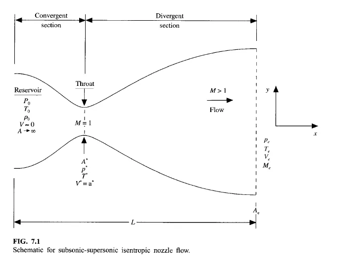
The flow from the inlet to the nozzle comes from a reservoir where the pressure and temperature as denoted by ρ0 & T0.

The cross-section area of the reservoir is large, A ---> ∞ and Velocity is small, V ---> 0

At the throat, the flow is locally subsonic in the convergent section of the nozzle, M=1 means that at this location, Velocity is equal to the local speed sound. V = V* = a* similarly pressure and temperature are denoted by ρ* & T*. The area is denoted by A*. Assuming the cross-section area A is uniform across that section and flow properties vary only in x direction.

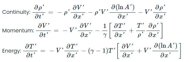
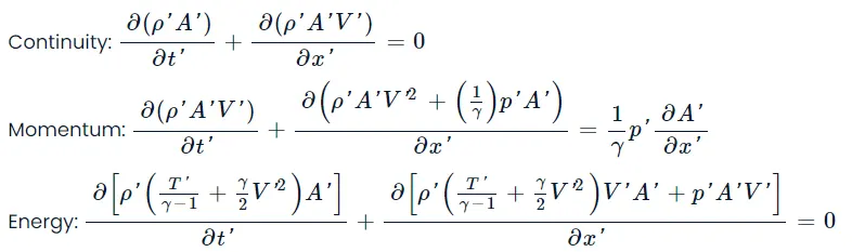
The Governing Continuity, Momentum and Energy equations for the Quasi-one-dimensional, Steady and Isentropic flow are given below.

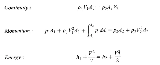
Subscript 1 & 2 denotes different locations along the nozzle.

From the Perfect gas equation of state, p=ρRT,

also Calorically perfect gas, h=CpT

The Mach number varies through the nozzle is governed by the area ratio A/A* through the relation

Here γ=1.4, standard condition of specific heats, Cp/Cv.

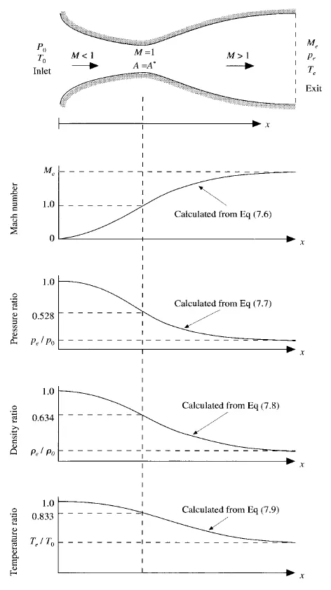
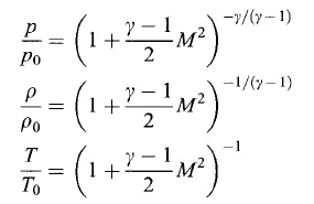
The variations of pressure, density and temperature as a function of Mach number are given below.

Governing Flow equations

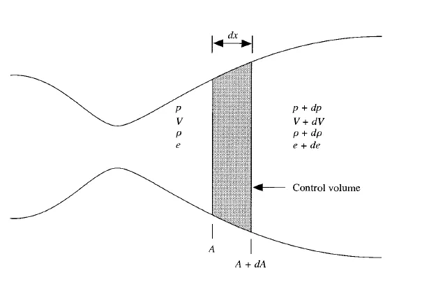
Here A + dx is the volume of the control volume in the limit of dx.

1. Nonconservation Form

2. Conservation Form

MacCormack's Technique

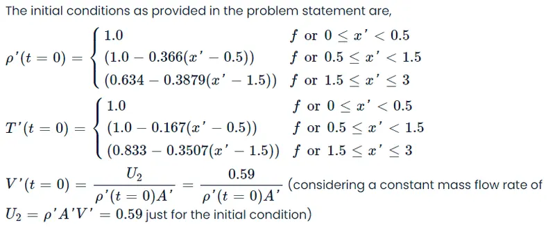
• Predictor Step - Forward difference scheme

• Corrective Step - Backward difference scheme

The continuity equation at the forward marching scheme can be obtained as below.

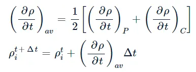
Similarly, Velocity & Temperature gradients are calculated.

1. Main Program

   clear all
   close all
   clc

   % solving Quasi 1-D super sonic nozzle flow equations for n nodes
   % In put parameter
   % No. of grid points
   n=31;

   gamma = 1.4
   x=linspace(0,3,n);
   dx = x(2)-x(1);

   % No. of timesteps
   nt = 1400
   % courant number
   c = 0.5;

   % function for non conservative form
   tic;
   [mass_flow_rate_ncf, pressure_ncf, mach_number_ncf, rho, v, t, rho_throat_ncf, v_throat_ncf, temp_throat_ncf, mass_flow_rate_throat_ncf, pressure_throat_ncf, mach_number_throat_ncf] = non_conservative_form(x,dx,n,gamma,nt,c);
   time = toc;
   fprintf('Simulation time for non conservative form = %0.4f',time);
   hold on

   % plotting
   % Timestep variation of properties at the throat area in non conservative
   % form

   figure(1)

   %Density
   subplot(4,1,1)
   plot(rho_throat_ncf,'color','r')
   ylabel('Density')
   legend({'Density at throat'});
   axis([0 1400 0 max(rho_throat_ncf)]);
   grid minor;
   title('Variation of field variables with respect to time step at throat area for non-conservative form')

   % Temperature
   subplot(4,1,2)
   plot(temp_throat_ncf,'color','c')
   ylabel('Temperature')
   legend({'Temperature at throat'});
   axis([0 1400 0.6 max(temp_throat_ncf)]);
   grid minor;

   
   % Pressure
   subplot(4,1,3)
   plot(pressure_throat_ncf,'color','c')
   ylabel('pressure')
   legend({'pressure at throat'});
   axis([0 1400 0.4 max(pressure_throat_ncf)]);
   grid minor;

   
   % Mach number
   subplot(4,1,4)
   plot(mach_number_throat_ncf,'color','r')
   xlabel('Timesteps')
   ylabel('pressure')
   legend({'Mach number at throat'});
   axis([0 1400 0.6 max(mach_number_throat_ncf)]);
   grid minor;

   
   % Steady state simulation for primitive values for non conservative form
   figure(2);

   %Density

   subplot(4,1,1)
   plot(x,rho,'color','m')
   ylabel('Densty')
   legend({'Density'});
   axis([0 3 0 max(rho)])
   grid minor;
   title('Variation of field variable along the length of nozzle for non-conservative form')

   % Temperature
   subplot(4,1,2)
   plot(x,t,'color','c')
   ylabel('Temperature')
   legend({'Temperature'});
   axis([0 3 0 max(t)])
   grid minor;

   % pressure
   subplot(4,1,3)
   plot(x,pressure_ncf,'color','g')
   ylabel('pressure')
   legend({'pressure'});
   axis([0 3 0 max(pressure_ncf)])
   grid minor;

   % Mach number
   subplot(4,1,4)
   plot(x,mach_number_ncf,'color','y')
   ylabel('Mach Number')
   legend({'Mach Number'});
   axis([0 3 0 max(mach_number_ncf)])
   grid minor;

   % function for conservative form
   tic;
   [mass_flow_rate_cf, pressure_cf, mach_number_cf, rho_cf, v_cf, temp_cf, rho_throat_cf, v_throat_cf, temp_throat_cf, mass_flow_rate_throat_cf, pressure_throat_cf, mach_number_throat_cf] = conservative_form(x,dx,n,gamma,nt,c);
   time = toc;
   fprintf('Simulation time for conservative form = %0.4f',time);
   hold on

   % plotting
   % Timestep variation of properties at the throat area in conservative form

   figure(3)

   % Density
   subplot(4,1,1)
   plot(rho_throat_cf,'color','m')
   ylabel('Density')
   legend({'Density at throat'});
   axis([0 1400 0.5 max(rho_throat_cf)]);
   grid minor;
   title('Variation of field variables with respect to time step at throat area for conservative form')

   % Temperature
   subplot(4,1,2)
   plot(temp_throat_cf,'color','c')
   ylabel('Temperature')
   legend({'Temperature at throat'});
   axis([0 1400 0.8 max(temp_throat_cf)]);
   grid minor;

   
   % Pressure
   subplot(4,1,3)
   plot(pressure_throat_cf,'color','g')
   ylabel('pressure')
   legend({'pressure at throat'});
   axis([0 1400 0.4 max(pressure_throat_cf)]);
   grid minor;

   % Mach number
   subplot(4,1,4)
   plot(mach_number_throat_cf,'color','y')
   xlabel('Timesteps')
   ylabel('Mach number')
   legend({'Mach number at throat'});
   axis([0 1400 0.9 max(mach_number_throat_cf)]);
   grid minor;

   % Steady state simulation for primitive values for non conservative form
   figure(4);

   % Density
   subplot(4,1,1)
   plot(x,rho_cf,'color','m')
   ylabel('Density')
   legend({'Density'});
   axis([0 3 0 max(rho_cf)])
   grid minor;
   title('Variation of flow rate distribution - conservative form')

   % Temperature
   subplot(4,1,2)
   plot(x,temp_cf,'color','c')
   ylabel('Temperature')
   legend({'Temperature'});
   axis([0 3 0 max(temp_cf)])
   grid minor;

   % pressure
   subplot(4,1,3)
   plot(x,pressure_cf,'color','g')
   ylabel('pressure')
   legend({'pressure'});
   axis([0 3 0 max(pressure_cf)])
   grid minor;

   % Mach number
   subplot(4,1,4)
   plot(x,mach_number_cf,'color','y')
   xlabel('Nozzle length')
   ylabel('Mach Number')
   legend({'Mach Number'});
   axis([0 3 0 max(mach_number_cf)])
   grid minor;

   % Comparison plot of normalized mass flow rate of both forms
   figure(5)
   hold on
   plot(x,mass_flow_rate_ncf,'r','linewidth',1)
   hold on
   plot(x,mass_flow_rate_cf,'b','linewidth',1)
   hold on
   grid on

   legend('Non-conservative','Conservative');
   xlabel('length of domain')
   ylabel('mass flow rate')
   title('Comparison of normalized mass flowrate of both forms')

2. Nonconservation Form

   function [mass_flow_rate_ncf, pressure_ncf, mach_number_ncf, rho, v, t, rho_throat_ncf, v_throat_ncf, temp_throat_ncf, mass_flow_rate_throat_ncf, pressure_throat_ncf, mach_number_throat_ncf] = non_conservative_form(x,dx,n,gamma,nt,c);

   % Calculate initial profiles
   rho = 1-0.3146*x;
   t = 1-0.2314*x; % t is a temperature
   v = (0.1+1.09*x).*t.^(1/2);

   % Area
   a = 1+2.2*(x-1.5).^2;
   throat = find(a==1)

   % outer time loop
   for k=1:nt
   
   %Time step control
   dt = min(c.*dx./(sqrt(t) + v));
   
   % Saving a copy of old values
   rho_old = rho;
   v_old = v;
   t_old = t;
   
   % predictor method
   for j = 2:n-1
   dvdx = (v(j+1)-v(j))/(dx);
   drhodx = (rho(j+1)-rho(j))/(dx);
   dtdx = (t(j+1)-t(j))/(dx);
   dlogadx = (log(a(j+1))-log(a(j)))/(dx);
   
   %continuity equation
   drhodt_p(j) = -rho(j)*dvdx - rho(j)*v(j)*dlogadx-v(j)*drhodx;
   
   %momentum equation
   dvdt_p(j) = -v(j)*dvdx - (1/gamma)*(dtdx+(t(j)/rho(j))*drhodx);
   
   % Energy equation
   dtdt_p(j) = -v(j)*dtdx -(gamma-1)*t(j)*(dvdx + v(j)*dlogadx);
   
   %solution update
   rho(j) = rho(j)+drhodt_p(j)*dt;
   v(j) = v(j)+dvdt_p(j)*dt;
   t(j) = t(j)+dtdt_p(j)*dt;
   end
   
   % corrector method
   for j = 2:n-1
   dvdx = (v(j)-v(j-1))/(dx);
   drhodx = (rho(j)-rho(j-1))/(dx);
   dtdx = (t(j)-t(j-1))/(dx);
   dlogadx = (log(a(j))-log(a(j-1)))/(dx);
   
   %continuity equation
   drhodt_c(j) = -rho(j)*dvdx - rho(j)*v(j)*dlogadx-v(j)*drhodx;
   
   %momentum equation
   dvdt_c(j) = -v(j)*dvdx - (1/gamma)*(dtdx+(t(j)/rho(j))*drhodx);
   
   % Energy equation
   dtdt_c(j) = -v(j)*dtdx -(gamma-1)*t(j)*(dvdx + v(j)*dlogadx);
   
   end
   
   % compute the average time derivation
   drhodt = 0.5*(drhodt_p + drhodt_c);
   dvdt = 0.5*(dvdt_p + dvdt_c);
   dtdt = 0.5*(dtdt_p + dtdt_c);
   
   % Final solution update
   for i=2:n-1
   v(i) = v_old(i) +dvdt(i)*dt;
   rho(i) = rho_old(i) +drhodt(i)*dt;
   t(i) = t_old(i)+dtdt(i)*dt;
   end
   
   %Apply boundary conditions
   % Inlet
   v(1) = 2*v(2) - v(3);
   
   %Outlet
   v(n) = 2*v(n-1)- v(n-2);
   rho(n) = 2*rho(n-1)- rho(n-2);
   t(n) = 2*t(n-1)- t(n-2);
   
   
   % Defining Mass flow rate, pressure and Mach number
   
   mass_flow_rate_ncf = rho.*a.*v;
   pressure_ncf = rho.*t;
   mach_number_ncf = (v./sqrt(t));
   
   % Calculating Variables at throat section
   rho_throat_ncf(k) = rho(throat);
   temp_throat_ncf(k) = t(throat);
   v_throat_ncf(k) = v(throat);
   mass_flow_rate_throat_ncf(k) = mass_flow_rate_ncf(throat);
   pressure_throat_ncf(k) = pressure_ncf(throat);
   mach_number_throat_ncf(k) = mach_number_ncf(throat);
   
   % plotting
   % comparison of non-dimensional mass flow rates at diferent time
   % steps
   
   figure(7)
   if k==50
   plot(x, mass_flow_rate_ncf,'m','linewidth',1);
   hold on
   elseif k == 100
   plot(x, mass_flow_rate_ncf,'c','linewidth',1);
   hold on
   elseif k == 200
   plot(x, mass_flow_rate_ncf,'g','linewidth',1);
   hold on
   elseif k == 400
   plot(x, mass_flow_rate_ncf,'y','linewidth',1);
   hold on
   elseif k == 800
   plot(x, mass_flow_rate_ncf,'k','linewidth',1);
   hold on
   end
   
   % Labelling
   title('Mass flow rates at different timesteps - non-conservative form')
   xlabel('Distance')
   ylabel('Mass flow rate')
   legend({'50th Timestep','100th Timestep','200th Timestep','400th Timestep','800th Timestep'})
   axis([0 3 0 2])
   grid on
   
   end

3. Conservation Form

   function [mass_flow_rate_cf, pressure_cf, mach_number_cf, rho_cf, v_cf, temp_cf, rho_throat_cf, v_throat_cf, temp_throat_cf, mass_flow_rate_throat_cf, pressure_throat_cf, mach_number_throat_cf] = conservative_form(x,dx,n,gamma,nt,c)

   % Determining initial profile of density or temperature
   for i=1:n
   
   if (x(i) >=0 && x(i) <=0.5)
   rho_cf(i) = 1;
   temp_cf(i) = 1;
   elseif (x(i) >=0.5 && x(i) <= 1.5)
   rho_cf(i) = 1-0.366*(x(i)-0.5);
   temp_cf(i) = 1 - 0.167*(x(i)-0.5);
   elseif (x(i) >=1.5 && x(i) <= 3)
   rho_cf(i) = 0.634-0.3879*(x(i)-1.5);
   temp_cf(i) = 0.833 - 0.3507*(x(i)-1.5);
   end
   end

   a = 1+2.2*(x-1.5).^2;
   throat = find(a==1);

   % Calculate initial profiles
   v_cf = 0.59./(rho_cf.*a);
   pressure_cf = rho_cf.*temp_cf;

   %Calculate the initial solution vectors(U)
   U1 = rho_cf.*a;
   U2 = U1.*v_cf;
   U3 = U1.*((temp_cf./(gamma-1))+(gamma/2).*(v_cf.^2));

   % Outer time loop
   for k =1:nt
   % Time-step control
   dt = min(c.*dx./(sqrt(temp_cf) + v_cf));
   % Dt = temp_c.^0.5;
   % dt = min(c*(dx./(Dt + v_c)));

   %saving a copy of old values
   U1_old = U1;
   U2_old = U2;
   U3_old = U3;
   
   %Calculating the flux vector(F)
   F1 = U2;
   F21 = (U2.^2)./(U1);
   F22 = (gamma-1)/(gamma);
   F23 = U3 - ((gamma/2).*F21);
   F2 = F21 + F22 * F23;

   
   F31 = (U2.*U3)./(U1);
   F32 = (gamma*(gamma-1))/2;
   F33 = (U2.^3)./(U1.^2);
   F3 = gamma.*F31 - (F32.*F33);

   
   
   % predictor method
   for j= 2:n-1
   
   % Calculating the source term(J)
   J2_P(j) = (1/gamma)*(rho_cf(j)*temp_cf(j))*((a(j+1)-a(j))/dx);
   
   % continuity equation
   dU1_dt_P(j) = -((F1(j+1)- F1(j))/dx);
   
   % Momentum equation
   dU2_dt_P(j) = -((F2(j+1)- F2(j))/dx)+J2_P(j);
   
   % Energy Equation
   dU3_dt_P(j) = -((F3(j+1) - F3(j))/dx);
   
   
   % Updating new values
   U1(j) = U1(j)+ dU1_dt_P(j)*dt;
   U2(j) = U2(j)+ dU2_dt_P(j)*dt;
   U3(j) = U3(j)+ dU3_dt_P(j)*dt;
   
   end
   
   % Updating flux vectors
   rho_cf = U1./a;
   v_cf = U2./U1;
   temp_cf = (gamma-1)*((U3./U1 - (gamma/2)*(v_cf).^2));
   
   %Calculating the flux vector(F)
   F1 = U2;
   F21 = (U2.^2)./(U1);
   F22 = (gamma-1)/(gamma);
   F23 = U3 - ((gamma/2).*F21);
   F2 = F21 + F22 * F23;

   
   F31 = (U2.*U3)./(U1);
   F32 = (gamma*(gamma-1))/2;
   F33 = (U2.^3)./(U1.^2);
   F3 = gamma.*F31 - (F32.*F33);
   
   
   %corrector Method
   for j = 2:n-1
   
   % updating the source term(J)
   J2(j) = (1/gamma)*rho_cf(j)*temp_cf(j)*((a(j)-a(j-1))/dx);
   
   %Simplifying the Equation's spatial terms
   dU1_dt_C(j) = -((F1(j)-F1(j-1))/dx);
   dU2_dt_C(j) = -((F2(j)-F2(j-1))/dx)+J2(j);
   dU3_dt_C(j) = -((F3(j)-F3(j-1))/dx);
   end
   
   % Compute Average time derivative
   dU1_dt = 0.5*( dU1_dt_P + dU1_dt_C);
   dU2_dt = 0.5*( dU2_dt_P + dU2_dt_C);
   dU3_dt = 0.5*( dU3_dt_P + dU3_dt_C);
   
   % Final solution update
   for i = 2:n-1
   U1(i) = U1_old(i) + dU1_dt(i)*dt;
   U2(i) = U2_old(i) + dU2_dt(i)*dt;
   U3(i) = U3_old(i) + dU3_dt(i)*dt;
   end
   
   % Applying Boundary conditions
   % At Inlet
   U1(1) = rho_cf(1)*a(1);
   U2(1) = 2*U2(2)-U2(3);
   
   v_cf(1) = U2(1)./U1(1);
   U3(1) = U1(1)*((temp_cf(1)/(gamma-1))+((gamma/2)*(v_cf(1)).^2));
   
   % At Outlet
   U1(n) = 2*U1(n-1)-U1(n-2);
   U2(n) = 2*U2(n-1)-U2(n-2);
   U3(n) = 2*U3(n-1)-U3(n-2);
   % Final primitive value update
   rho_cf = U1./a;
   v_cf = U2./U1;
   temp_cf = (gamma-1)*((U3./U1 - (gamma/2)*(v_cf).^2));
   
   % Defining Mass flow rate, pressure and Mach number
   
   mass_flow_rate_cf = rho_cf.*a.*v_cf;
   pressure_cf = rho_cf.*temp_cf;
   mach_number_cf = (v_cf./sqrt(temp_cf));
   
   % Calculating Variables at throat section
   rho_throat_cf(k) = rho_cf(throat);
   temp_throat_cf(k) = temp_cf(throat);
   v_throat_cf(k) = v_cf(throat);
   mass_flow_rate_throat_cf(k) = mass_flow_rate_cf(throat);
   pressure_throat_cf(k) = pressure_cf(throat);
   mach_number_throat_cf(k) = mach_number_cf(throat);
   
   % plotting
   % comparison of non-dimensional mass flow rates at diferent time
   % steps
   
   figure(6)
   if k==50
   plot(x, mass_flow_rate_cf,'m','linewidth',1);
   hold on
   elseif k == 100
   plot(x, mass_flow_rate_cf,'c','linewidth',1);
   hold on
   elseif k == 200
   plot(x, mass_flow_rate_cf,'g','linewidth',1);
   hold on
   elseif k == 400
   plot(x, mass_flow_rate_cf,'y','linewidth',1);
   hold on
   elseif k == 800
   plot(x, mass_flow_rate_cf,'k','linewidth',1);
   hold on
   end
   
   % Labelling
   title('Mass flow rates at different timesteps - conservative form')
   xlabel('Distance')
   ylabel('Mass flow rate')
   legend({'50th Timestep','100th Timestep','200th Timestep','400th Timestep','800th Timestep'})
   axis([0 3 0.4 1])
   grid on
   
   end
   end

Values of Density, Velocity and Temperature for node, N=31 & 61

Primate variables and conditions at nozzle

		Density ratio ρ/ρo	Temperature ratio T/To	Pressure ratio P/Po	Mach number M
n=31	non conservative	0.6387	0.8365	0.5342	0.9994
n=61	non conservative	0.6377	0.8354	0.5327	0.9998
n=31	conservative	0.6642	0.8939	0.5937	0.9801
n=61	conservative	0.6424	0.8601	0.5525	1.0008

Exact solution

0.634

0.833

0.528

1.00

Simulation time data:

grid points		time for simulation
n=31	non conservative	3.1510
n=31	conservative	2.952
n=61	non conservative	3.2231
n=61	conservative	3.0038

CFL data effect on non-coservative form for 31 grid points:

CFL number	Density ratio ρ/ρo	Temperature ratio T/To	Pressure ratio P/Po	Mach number M
0.5	0.6387	0.8365	0.5342	0.9994
0.8	0.6393	0.8367	0.5349	0.9991
1.0	0.6397	0.8368	0.5353	0.9988
1.1	0.6399	0.8369	0.5355	0.9987
1.2	----------	-----------	-----------	--------

Exact solution

0.634

0.833

0.528

1.00

The solution blew at CFL value equal to 1.2

CFL data effect on conservative form for 31 grid points:

CFL number	Density ratio ρ/ρo	Temperature ratio T/To	Pressure ratio P/Po	Mach number M
0.5	0.6642	0.8939	0.5937	0.9801
0.8	0.6642	0.8939	0.5937	0.9801
1.0	0.6642	0.8939	0.5937	0.9801
1.1	0.6642	0.8939	0.5937	0.9801
1.2	0.6642	0.8939	0.5937	0.9801

Exact solution

0.634

0.833

0.528

1.00

Conclusion:

• MacCormack's technique is a variant of the Lax-Wendroff approach.
• It is an Explicit finite difference technique.
• The second order is accurate in both space and time.
• Mostly, easy to program.