Week 5.1 - Mid term project - Solving the steady and unsteady 2D heat conduction problem

AIM:- To Solve the steady and unsteady 2D heat conduction problem using the Iterative method

Objective:-

• To perform Steady-state analysis & Transient (Unsteady) State Analysis.
• To understand the different iterative techniques used to solve the steady and unsteady 2D heat conduction problem

Theory:-

Heat conduction is defined as The process by which heat is transferred from the hotter end to the colder end of the object.

The heat conduction equation is a second-order partial differential equation that describes the distribution of heat energy in a given body over time.

2D heat conduction

∂²T/∂t²+α(∂²T/∂x²+∂²T/∂y²)=0

STEADY-STATE 2D HEAT CONDUCTION

In a steady-state heat transfer, the heat flow rate remains constant at any point in time. Steady-state heat transfer can be described in terms of the temperature as the variable; the temperature of the system remains constant over time in steady-state heat transfer after thermal equilibrium is attained.

∂²T/∂x²+∂²T/∂y²=0

We can discretize the above equation into an algebraic form so that it can be used for computation,

For discretization, it can be assumed as

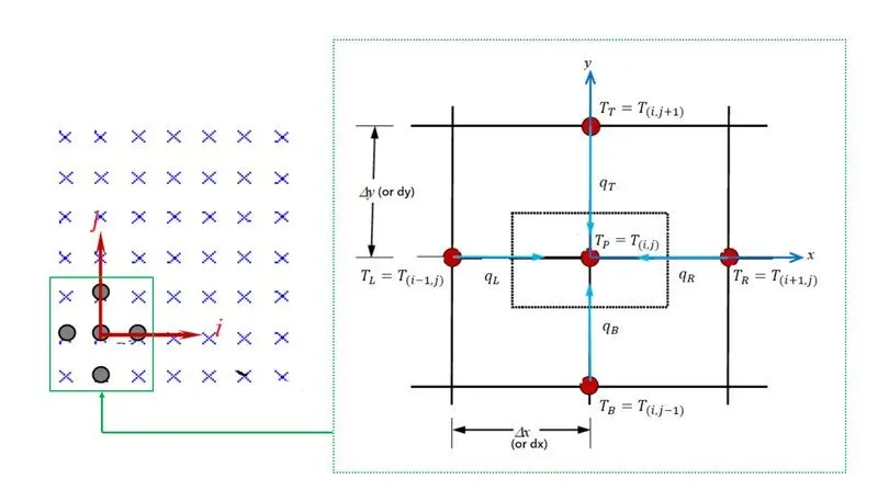
T_p = T_i,j - Current point for which calculating

T_R=T_i+1,j - Point on the right of the current point

T_L=T_i−1,j - Point on the right of the current point

T_T=T_i,j+1 - Top point of current point

T_B=T_i,j−1 - Bottom point of the current point

Now the Equation can be written as,

⇒Ti+1,j−2Ti,j+Ti−1,jdx2+Ti,j+1−2Ti,j+Ti,j−1dy2=0

⇒TR−2TP+TLdx2+TT−2TP+TBdy2=0

On Rearranging,

⇒Tp=dy22.(dx2+dy2).(TR+TL)+dx22.(dx2+dy2).(TT+TB)

Considering,

KX=dy22.(dx2+dy2)KX=dy22.(dx2+dy2) and
KY=dx22.(dx2+dy2)KY=dx22.(dx2+dy2)

Therefore,

TP=KX.(TR+TL)+KY.(TT+TB)TP

Transient state 2D heat conduction-

Transient heat transfer can also be called unsteady-state heat transfer. This type of heat transfer only exists for a short duration of time. In transient heat transfers, the heat energy transferred through the medium is not constant. The heat flow rate keeps changing, and the cause of the varying rates of heat transfer can be either fluctuating temperature differences over the medium or changes in properties of the medium.

In the physical world, heat transfer starts as transient and then reaches a steady state until thermal equilibrium is reached.

∂2T∂t2+α(∂2T∂x2+∂2T∂y2)=0

Where αα is the thermal diffusivity

We can discretize the above equation into an algebraic form so that it can be used for computation,

⇒Tn+1i,j−Tni,jdt+α.(Ti+1,j−2Ti,j+Ti−1,jdx2+Ti,j+1−2Ti,j+Ti,j−1dy2)=0

⇒TNP−TOPdt+α.(TOR−2TOP+TOLdx2+TOT−2TOP+TOBdy2=0

⇒TNP=TOP+α.dt(TOR−2TOP+TOLdx2+TOT−2TOP+TOBdy2)

Here, the current time step (i.e. at n) is shown by a suffix of 'O' representing Old-time, and the next time step (i.e. n+1) is by a suffix of 'N'

considering,

KXT=α.dtdx2KXT=α.dtdx2 and

KYT=α.dtdy2KYT=α.dtdy2

Therefore,

Implicit,

TNP=TOP+KXT.(TOR−2TOP+TOL)+KYT.(TOT−2TOP+TOBTNP

Explicit,

TNP=TOP+KXT.(TNR−2TNP+TNL)+KYT.(TNT−2TNP+TNBTNP

Iterative Solver:

1. Jacobi method- In this method, the temperature at (n+1) iteration is found using old values of the temperature defined at nth iterations. Using the approximation obtained iteration procedure is continued until the desired accuracy of the solution is obtained.
2. Gauss-Seidel method- In this type of iterative solver, the temperature at n+1 iterations uses values of n+1 iterations that have already been computed. In this way, old approximated values are overwritten with new approximate values for the iterations performed. Unlike Jacobi, Gauss seidel requires one storage vector which can be overwritten with each computation.
3. Successive over-relaxation method- In this type of iterative solver relaxation factor is used which helps in increasing the convergence rate. It goes by the formula

Tn+1 = Tn(1-w)+T(GS)

where w is between O-1 it is called under relaxed state.

This condition is used when the temperature gradient is low and due to this condition larger time steps are used to obtain the steady-state i.e., for the values to converge at a faster rate

Tn">Tn is the value of temperature for previous iterations.

T(GS) or T(Jacobi) is the temperature of value for (n+1) iteration using gauss seidel or Jacobi iterative solver.

THERMAL DIFFUSIVITY AND CFL CRITERIA -

The Thermal Diffusivity (αα) is an important factor in the solution, as it is related to the CFL Criteria shown below,

CFL = (α.dt)(1∂x2+1∂y2)=0

Thermal Diffusivity of material is an important factor and is interrelated with the dt, dx, and the CFL number. There will be an optimum CFL i.e. optimum value of it, dx, and dy.
For the smaller value of the αα the size of it will be higher to maintain stability i.e. here CFL no., but it reduces the accuracy of the solution, and for the larger value of αα the size of it will be small for the optimum CFL, but it can increase the simulation time. Since the implicit method is unconditionally stable at any time step value, the CFL condition can still be used to determine the optimum 'it' to maintain time accuracies.

% Main Program %
close all
clear all
clc

% Steady State Heat Conduction || (d^2T/dx^2 + d^2T/dy^2 = 0)

nx = 10;
ny = 10;

T = 450*ones(nx,ny);

TL = 400;
TR = 800;
TT = 600;
TB = 900;

% Boundary Conditions
T(:,1) = TL;
T(:,ny) = TR;
T(1,:) = TT;
T(nx,:) = TB;

% Edge Refinement
T(1,1) = (T(1,2)+T(2,1))/2;
T(1,ny) = (T(1,(ny-1))+T(2,ny))/2;
T(nx,1) = (T((nx-1),1)+T(nx,2))/2;
T(nx,ny) = (T(nx,(ny-1))+T((nx-1),ny))/2;

% Saving a Copy
Told = T;
T_initial = T;
error = 9e9;
tol = 1e-4;

% Iteration Solvers - Jacobi , GS & SOR Methods

% 1 --- Jacobi Method

jacobi_iteration = 0;
while (error > tol)

for i = 2:nx-1
for j = 2:ny-1

T(i,j) = 0.25*(Told(i+1,j) + Told(i-1,j) +Told(i,j+1) + Told(i,j-1));

end
end

error = max(max(abs(T-Told)));
Told = T;
jacobi_iteration = jacobi_iteration +1;

figure(1)
contourf(flipud(T),'ShowText','ON')
title(sprintf('Steady State Jacobi Iteration = %d',jacobi_iteration));


end
colorbar

% Reinitialising
T = T_initial;
Told = T;
error = 9e9;

% 2 --- Gauss Seidel (GS) Method

gaus_iteration = 0;
while (error > tol)

for i = 2:nx-1
for j = 2:ny-1

T(i,j) = 0.25*(Told(i+1,j) + T(i-1,j) +Told(i,j+1) + T(i,j-1));

end
end

error = max(max(abs(T-Told)));
Told = T;
gaus_iteration = gaus_iteration +1;


figure(2)
contourf(flipud(T),'ShowText','ON')
title(sprintf('Steady State Gauss Seidel Iteration= = %d',gaus_iteration));
pause(0.003)

end
colorbar

% Reinitialising
T = T_initial;
Told = T;
error = 9e9;

% 3 --- Successive over-relaxation(SOR) Method

sor_iteration = 0;
omega = 1.5;

while (error > tol)

for i = 2:nx-1
for j = 2:ny-1

TGS(i,j) = 0.25*(Told(i+1,j) + T(i-1,j) + T(i,j-1) +Told(i,j+1));
T(i,j) = (1-omega)*Told(i,j) + omega*TGS(i,j);


end
end

error = max(max(abs(T-Told)));
Told = T;
sor_iteration = sor_iteration +1;


figure(3)
contourf(flipud(T),'ShowText','ON')
title(sprintf('Steady State Successive over-relaxation Iteration= = %d',sor_iteration));
pause(0.003)

end
colorbar

% Program for Transient-State 2D Heat Conduction using Explicit Method %

close all
clear all
clc

% Transient State Heat Conduction
% dt^2/dT^2 + aplha(d^2T/dx^2 + d^2T/dy^2)=0

nx = 10;
ny = 10;

T = 450*ones(nx,ny);

TL = 400;
TR = 800;
TT = 600;
TB = 900;

% Boundary Conditions
T(:,1) = TL;
T(:,ny) = TR;
T(1,:) = TT;
T(nx,:) = TB;

% Edge Refinement
T(1,1) = (T(1,2)+T(2,1))/2;
T(1,ny) = (T(1,(ny-1))+T(2,ny))/2;
T(nx,1) = (T((nx-1),1)+T(nx,2))/2;
T(nx,ny) = (T(nx,(ny-1))+T((nx-1),ny))/2;

% Inputs
% Time Step
dt = 1e-2;
% Grid Spacing
dx = 1.3e-2;
dy = 1.3e-2;
% Thermal Diffusibility
alpha = 0.004;

k1 = alpha*dt/dx^2;
k2 = alpha*dt/dy^2;

cfl = k1 + k2

% Copy of previous result %
T_previous = T;

conv = 9e9;
tol = 1e-4;

time_iteration = 0;

% Time Looping %
while (conv > tol)

for i = 2:nx-1
for j = 2:ny-1

T(i,j) = (1-2*k1-2*k2)*T_previous(i,j) + k1*(T_previous(i+1,j)+ T_previous(i-1,j)) +k2*(T_previous(i,j+1) + T_previous(i,j-1));

end
end

conv = max(max(abs(T-T_previous)));
T_previous = T;
time_iteration = time_iteration +1;

figure(1)
contourf(flipud(T),'ShowText','ON')
title(sprintf('Transient Explicit Iteration = %d',time_iteration));
pause(0.003)

end
colorbar

% Program for Transient-State 2D Heat Conduction using Explicit Method %

close all
clear all
clc

% Transient State Heat Conduction
% dt^2/dT^2 + aplha(d^2T/dx^2 + d^2T/dy^2) = 0)
nx = 10;
ny = 10;

T = 450*ones(nx,ny);

TL = 400;
TR = 800;
TT = 600;
TB = 900;

% Boundary Conditions
T(:,1) = TL;
T(:,ny) = TR;
T(1,:) = TT;
T(nx,:) = TB;

% Edge Refinement
T(1,1) = (T(1,2)+T(2,1))/2;
T(1,ny) = (T(1,(ny-1))+T(2,ny))/2;
T(nx,1) = (T((nx-1),1)+T(nx,2))/2;
T(nx,ny) = (T(nx,(ny-1))+T((nx-1),ny))/2;

% Inputs from Assesment %
% Time Step for iterations
dt = 1e-2;
% Grid Spacing for accurate results
dx = 1e-2;
dy = 1e-2;
% Thermal Diffusibility constant
alpha = 1.5;

k1 = alpha*dt/dx^2
k2 = alpha*dt/dy^2

% Saving a Copy
Told = T;
T_initial = T;
T_prev = T;

error = 9e9;
conv = 9e9;
tol = 1e-4;

% Iteration Solvers - Jacobi || GS || SOR

% 1- Jacobi Method

jacobi_iteration = 0;
jacobi_time_iterations = 0;

% Time Loop for iterations %
while (conv > tol)

% Space Loop
while (error > tol)

for i = 2:nx-1
for j = 2:ny-1

T(i,j) = (1+2*k1+2*k2)^-1 *(T_prev(i,j)+ k1*(Told(i+1,j)+ Told(i-1,j)) +k2*(Told(i,j+1) + Told(i,j-1)));

end
end

error = max(max(abs(T-Told)));
Told = T;
jacobi_iteration = jacobi_iteration +1;

figure(1)
contourf(flipud(T),'ShowText','ON')
title(sprintf('Transient Implicit Jacobi Iteration = %d \n Time Iteration = %d',jacobi_iteration,jacobi_time_iterations));
pause(0.003)

end
conv = max(max(abs(T-T_prev)));
T_prev = T;
jacobi_time_iterations = jacobi_time_iterations +1;
error = 9e9;

end
colorbar

% Reinitialising the old values %
T = T_initial;
Told = T;
T_prev = T;
error = 9e9;
conv = 9e9;

% 2 ------ Gauss Seidel Method %

gs_iteration = 0;
gs_time_iteration =0;
% Time Loop
while (conv > tol)

% Space Loop
while (error > tol)

for i = 2:nx-1
for j = 2:ny-1

T(i,j) = (1+2*k1+2*k2)^-1 *(T_prev(i,j)+ k1*(Told(i+1,j)+ T(i-1,j)) +k2*(Told(i,j+1) + T(i,j-1)));

end
end

error = max(max(abs(T-Told)));
Told = T;
gs_iteration = gs_iteration +1;

figure(2)
contourf(flipud(T),'ShowText','ON')
title(sprintf('Transient Implicit Gauss Siedel Iteration = %d \n Time Iteration = %d',gs_iteration,gs_time_iteration));
pause(0.003)

end
conv = max(max(abs(T-T_prev)));
T_prev = T;
gs_time_iteration = gs_time_iteration +1;
error = 9e9;

end
colorbar

% Reinitialising
T = T_initial;
Told = T;
T_prev = T;
error = 9e9;
conv = 9e9;

% 3- Successive over-relaxation (SOR)

sor_iteration = 0;
sor_time_iteration = 0;
omega = 1.5;

% Time Loop
while (conv > tol)

% Space Loop
while (error > tol)

for i = 2:nx-1
for j = 2:ny-1

TGS(i,j) = (1+2*k1+2*k2)^-1 *(T_prev(i,j)+ k1*(Told(i+1,j)+ T(i-1,j)) +k2*(Told(i,j+1) + T(i,j-1)));
T(i,j) = (1-omega)*Told(i,j) + omega*TGS(i,j);

end
end

error = max(max(abs(T-Told)));
Told = T;
sor_iteration = sor_iteration +1;

figure(3)
contourf(flipud(T),'ShowText','ON')
title(sprintf('Transient Implicit Successive over-relaxation Iteration = %d \n Time Iteration = %d',sor_iteration,sor_time_iteration));
pause(0.003)

end
conv = max(max(abs(T-T_prev)));
T_prev = T;
sor_time_iteration = sor_time_iteration +1;
error = 9e9;

end
colorbar

Matlab Programs and Outputs are attached.