Week 3.5 - Deriving 4th order approximation of a 2nd order derivative using Taylor Table method

• AIM:

The main aim of the challenge is to derive the 4th order approximation of second order derivative using center difference,Right side skewed and Left side skewed methods.

• OBJECTIVE:

CENTER DIFFERENCE SCHEME:

For center difference scheme numerical stencil will be,

`(del^2f)/(delx^2)=af(i-2)+bf(i-1)+cf(i)+df(i+1)+ef(i+2)`

Taylor's series expansion for each term,

`af(i-2)=a(f(i)+(-2Deltax)f'(i) +(-2Deltax)^2/(2!)f''(i)+(-2Deltax)^3/(3!)f'''(i)+(-2Deltax)^4/(4!)f''''(i)+(-2Deltax)^5/(5!)f'''''(i)+............)`

`bf(i-1)=b(f(i)+(-Deltax)f'(i) +(-Deltax)^2/(2!)f''(i)+(-Deltax)^3/(3!)f'''(i)+(-Deltax)^4/(4!)f''''(i)+(-Deltax)^5/(5!)f'''''(i)+............)`

`cf(i)=cf(i)`

`df(i+1)=d(f(i)+(Deltax)f'(i) +(Deltax)^2/(2!)f''(i)+(Deltax)^3/(3!)f'''(i)+(Deltax)^4/(4!)f''''(i)+(Deltax)^5/(5!)f'''''(i)+............)`

`ef(i+2)=e(f(i)+(2Deltax)f'(i) +(2Deltax)^2/(2!)f''(i)+(2Deltax)^3/(3!)f'''(i)+(2Deltax)^4/(4!)f''''(i)+(2Deltax)^5/(5!)f'''''(i)+............)`

By arranging the above Taylor's expansion in Taylor's table we get,

	`f(i)`	`Deltaxf'(i)`	`Deltax^2f''(i)`	`Deltax^3f'''(i)`	`Deltax^4f''''(i)`	`Deltax^5f'''''(i)`	`Deltax^6f''''''(i)`
`af(i-2)`	a	-2a	4a/2	-8a/6	16a/24	-32a/120	64a/720
`bf(i-1)`	b	-b	b/2	-b/6	b/24	-b/120	b/720
`cf(i)`	c	0	0	0	0	0	0
`df(i+1)`	d	d	d/2	d/6	d/24	d/120	d/720
`ef(i+2)`	e	2e	4e/2	8e/6	16e/24	-32e/120	64e/720
`(Deltax^2)*(del^2f)/(delx^2)`	0	0	1	0	0	?	?

Here we have 5 unknowns and 5 equation's can be solved by system of linear equation in MATLAB and find the value of a,b,c,d,e

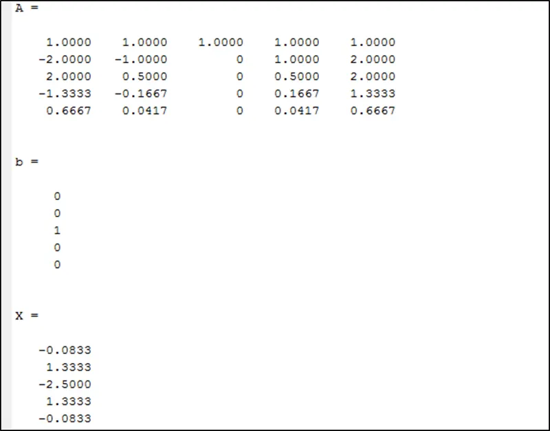
a=-0.0833

b=1.3333

c= -2.5000

d=1.3333

e=-0.0833

by putting the values of coefficient we will get 4th order approximation of second order center difference method,

`(del^2f)/(delx^2)=(((-0.0833)f(i-2)+(1.3333)f(i-1)+(-2.5)f(i)+(1.3333)f(i+1)+(-0.0833)f(i+2))/(Deltax^2))`

From the above values we can say that a=e,b=d

so,-32a/120-b/120+d/120-32e/120 = 0

Then,

`(Deltax^2)(del^2f)/(delx^2)` = (4a/2+b/2+d/2+4e/2)`Deltax^2f''(i)`+(64a/720+b/720+d/720+64e/720)`Deltax^6f''''''(i)`

Now divide the above equation with `(Deltax)^2` we get

`(del^2f)/(delx^2)` = (4a/2+b/2+d/2+4e/2)`f''(i)`+(64a/720+b/720+d/720+64e/720)`Deltax^4f''''''(i)`

In the above equation `Deltax^4` represents the truncation error,therefore we can say that center difference is 4th order accurate.

SKEWED RIGHTSIDE DIFFERENCE SCHEME:

For skewed rightside difference scheme numerical stencil will be,

`(del^2f)/(delx^2)=af(i)+bf(i+1)+cf(i+2)+df(i+3)+ef(i+4)+gf(i+5)`

Taylor's series expansion for each term,

`af(i)=af(i)`

`bf(i+1)=b(f(i)+(Deltax)f'(i) +(Deltax)^2/(2!)f''(i)+(Deltax)^3/(3!)f'''(i)+(Deltax)^4/(4!)f''''(i)+(Deltax)^5/(5!)f'''''(i)+............)`

`cf(i+2)=c(f(i)+(2Deltax)f'(i) +(2Deltax)^2/(2!)f''(i)+(2Deltax)^3/(3!)f'''(i)+(2Deltax)^4/(4!)f''''(i)+(2Deltax)^5/(5!)f'''''(i)+............)`

`df(i+3)=d(f(i)+(3Deltax)f'(i) +(3Deltax)^2/(2!)f''(i)+(3Deltax)^3/(3!)f'''(i)+(3Deltax)^4/(4!)f''''(i)+(3Deltax)^5/(5!)f'''''(i)+............)`

`ef(i+4)=e(f(i)+(4Deltax)f'(i) +(4Deltax)^2/(2!)f''(i)+(4Deltax)^3/(3!)f'''(i)+(4Deltax)^4/(4!)f''''(i)+(4Deltax)^5/(5!)f'''''(i)+............)`

`gf(i+5)=g(f(i)+(5Deltax)f'(i) +(5Deltax)^2/(2!)f''(i)+(5Deltax)^3/(3!)f'''(i)+(5Deltax)^4/(4!)f''''(i)+(5Deltax)^5/(5!)f'''''(i)+............)`

By arranging the above Taylor's expansion in Taylor's table we get,

	`f(i)`	`Deltaxf'(i)`	`Deltax^2f''(i)`	`Deltax^3f'''(i)`	`Deltax^4f''''(i)`	`Deltax^5f'''''(i)`	`Deltax^6f''''''(i)`
`af(i)`	a	0	0	0	0	0	0
`bf(i+1)`	b	b	b/2	b/6	b/24	b/120	b/720
`cf(i+2)`	c	2c	4c/2	8c/6	16c/24	32c/120	64c/720
`df(i+3)`	d	3d	9d/2	27d/6	81d/24	243d/120	729d/720
`ef(i+4)`	e	4e	16e/2	64e/6	256e/24	1024e/120	4096e/720
`gf(i+5)`	g	5g	25g/2	125g/6	625g/24	3125g/120	15625g/720
`(Deltax^2)*(del^2f)/(delx^2)`	0	0	1	0	0	0	?

Here we have 6 unknowns and 6 equation's can be solved by system of linear equation in MATLAB and find the value of a,b,c,d,e,g

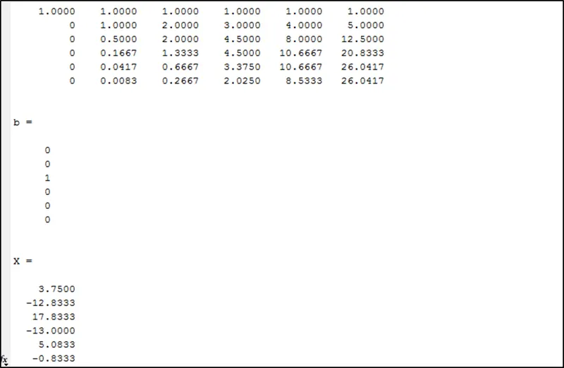
a=3.7500

b=-12.8333

c=17.8333

d=-13.0000

e=5.0833

g=-0.8333

by putting the values of coefficient we will get 4th order approximation of second order skewed rightside difference method,

`(del^2f)/(delx^2)=((3.75)f(i)+(-12.8333)f(i+1)+(17.8333)f(i+2)+(-13.0)f(i+3)+(5.0833)f(i+4)+(-0.8333)f(i+5))/(Deltax^2))`

from Taylor's table we get,

`(Deltax^2)*(del^2f)/(delx^2)`= (b/2+4c/2+9d/2+16e/2+25g/2)`Deltax^2f''(i)`+(b/720+64c/720+729d/720+4096e/720+15625g/720)`Deltax^6f''''''(i)`

then

`(del^2f)/(delx^2)`= (b/2+4c/2+9d/2+16e/2+25g/2)+(b/720+64c/720+729d/720+4096e/720+15625g/720)`Deltax^4f''''''(i)`

In the above equation `Deltax^4` represents the truncation error,therefore we can say that Skewed Rightside difference is 4th order accurate.

SKEWED LEFTSIDE DIFFERENCE SCHEME:

For skewed rightside difference scheme numerical stencil will be,

`(del^2f)/(delx^2)=af(i-5)+bf(i-4)+cf(i-3)+df(i-2)+ef(i-1)+gf(i)`

Taylor's series expansion for each term,

`af(i-5)=a(f(i)+(-5Deltax)f'(i) +(-5Deltax)^2/(2!)f''(i)+(-5Deltax)^3/(3!)f'''(i)+(-5Deltax)^4/(4!)f''''(i)+(-5Deltax)^5/(5!)f'''''(i)+............)`

`bf(i-4)=b(f(i)+(-4Deltax)f'(i) +(-4Deltax)^2/(2!)f''(i)+(-4Deltax)^3/(3!)f'''(i)+(-4Deltax)^4/(4!)f''''(i)+(-4Deltax)^5/(5!)f'''''(i)+............)`

`cf(i-3)=c(f(i)+(-3Deltax)f'(i) +(-3Deltax)^2/(2!)f''(i)+(-3Deltax)^3/(3!)f'''(i)+(-3Deltax)^4/(4!)f''''(i)+(-3Deltax)^5/(5!)f'''''(i)+............)`

`df(i-2)=d(f(i)+(-2Deltax)f'(i) +(-2Deltax)^2/(2!)f''(i)+(-2Deltax)^3/(3!)f'''(i)+(-2Deltax)^4/(4!)f''''(i)+(-2Deltax)^5/(5!)f'''''(i)+............)`

`ef(i-1)=e(f(i)+(-Deltax)f'(i) +(-Deltax)^2/(2!)f''(i)+(-Deltax)^3/(3!)f'''(i)+(-Deltax)^4/(4!)f''''(i)+(-Deltax)^5/(5!)f'''''(i)+............)`

`gf(i)=gf(i)`

By arranging the above Taylor's expansion in Taylor's table we get,

	`f(i)`	`Deltaxf'(i)`	`Deltax^2f''(i)`	`Deltax^3f'''(i)`	`Deltax^4f''''(i)`	`Deltax^5f'''''(i)`	`Deltax^6f''''''(i)`
`af(i-5)`	a	-5a	25a/2	-125a/6	625a/24	-3125a/120	15625a/720
`bf(i-4)`	b	-4b	8b	-64b/6	256b/24	-1024b/120	4096b/720
`cf(i-3)`	c	-3c	9c/2	-27c/6	81c/24	-243c/120	729c/720
`df(i-2)`	d	-2d	2d	-8d/6	16d/24	-32d/120	64d/720
`ef(i-1)`	e	-e	e/2	-e/6	e/24	-e/120	e/720
`gf(i)`	g	0	0	0	0	0	0
`(Deltax^2)*(del^2f)/(delx^2)`	0	0	1	0	0	0	?

Here we have 6 unknowns and 6 equation's can be solved by system of linear equation in MATLAB and find the value of a,b,c,d,e,g

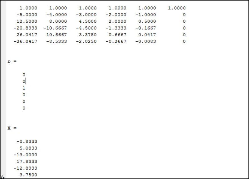
a=-0.8333

b=5.0833

c=-13.00

d=17.8333

e=-12.8333

g=3.7500

by putting the values of coefficient we will get 4th order approximation of second order skewed leftside difference method,

`(del^2f)/(delx^2)=((-0.8333)f(i-5)+(5.0833)f(i-4)+(-13.000)f(i-3)+(17.8333)f(i-2)+(-12.8333)f(i+1)+(3.7500)f(i))/(Deltax^2)`

from Taylor's table we get,

`(Deltax^2)*(del^2f)/(delx^2)`=(25a/2+8b+9c/2+2d+e/2)`Deltax^2f''(i)`+(15625a/720+4096b/720+729c/720+64d/720+e/720)`Deltax^6f''''''(i)`

then,

`(del^2f)/(delx^2)`=(25a/2+8b+9c/2+2d+e/2)+(15625a/720+4096b/720+729c/720+64d/720+e/720)`Deltax^4f''''''(i)`

In the above equation `Deltax^4` represents the truncation error,therefore we can say that Skewed Leftside difference is 4th order accurate.

• CODING:

CENTER DIFFERENCE FUNCTION:

function out = center_differencing_scheme(x,dx)

%Analytical derivative of function f(x) = exp(x)*cos(x)
Analytical_derivative = -2*exp(x)*sin(x);

a = -0.083333;
b = 1.333333;
c = -2.500000;
d = 1.333333;
e = -0.083333;

%Center difference scheme

center_difference_approx = (a*(exp(x-2*dx)*cos(x-2*dx))+b*(exp(x-dx)*cos(x-dx))+c*(exp(x)*cos(x))+d*(exp(x+dx)*cos(x+dx))+e*(exp(x+2*dx)*cos(x+2*dx)))/(dx)^2;

 out = abs(center_difference_approx-Analytical_derivative);

end

SKEWED RIGHTSIDE DIFFERENCE:

function out = Skewed_rightside_difference(x,dx)

%Analytical derivative of function f(x) = exp(x)*cos(x)
Analytical_derivative = -2*exp(x)*sin(x);

a = 3.75000;
b = -12.83333;
c = 17.83333;
d = -13.00000;
e = 5.08333;
g = -0.83333;

%Skewed Rightside Difference Scheme

Skewed_rightside_approx = (a*(exp(x)*cos(x))+b*(exp(x+dx)*cos(x+dx))+c*(exp(x+2*dx)*cos(x+2*dx))+ d*(exp(x+3*dx)*cos(x+3*dx))+e*(exp(x+4*dx)*cos(x+4*dx))+g*(exp(x+5*dx)*cos(x+5*dx)))/(dx)^2;

out = abs(Skewed_rightside_approx-Analytical_derivative);

end

SKEWED LEFTSIDE DIFFERENCE :

function out = Skewed_leftside_difference(x,dx)

%Analytical derivative of function f(x) = exp(x)*cos(x)
Analytical_derivative = -2*exp(x)*sin(x);

g = 3.75000;
e = -12.83333;
d = 17.83333;
c = -13.00000;
b = 5.08333;
a = -0.83333;

%Skewed Leftside Difference Scheme

Skewed_leftside_approx = (a*(exp(x-5*dx)*cos(x-5*dx))+b*(exp(x-4*dx)*cos(x-4*dx))+c*(exp(x-3*dx)*cos(x-3*dx))+d*(exp(x-2*dx)*cos(x-2*dx))+e*(exp(x-1*dx)*cos(x-1*dx))+g*exp(x)*cos(x))/(dx)^2;

out = abs(Skewed_leftside_approx-Analytical_derivative);
 
end

MAIN PROGRAM:

clear all
close all
clc

%Initial values
x= pi/3;
dx = linspace(pi/4,pi/400,40);

for i = 1:length(dx)
   center_difference_error(i) = center_differencing_scheme(x,dx(i));
   skewed_rightside_error(i) = Skewed_rightside_difference(x,dx(i));
   skewed_leftside_error(i)= Skewed_leftside_difference(x,dx(i));
   
end

%Plotting
figure(1)
loglog(dx,center_difference_error)
hold on
loglog(dx,skewed_rightside_error)
hold on
loglog(dx,skewed_leftside_error)
xlabel('step size(dx)')
ylabel('Error')
legend('center difference error','skewed rightside error','skewed leftside error')
title('Fourth order approximation of second order derivative')

• EXPLANATION:

1. Initialize the code with clear all,close all and clc to clear all the previous data stored in workspace.
2. Set the initial values of x and range of dx using linspace command.
3. Call the created function inside a for loop which calculate the value of error for each value of dx.
4. In function program give all the coefficient values which is calculated in MATLAB.
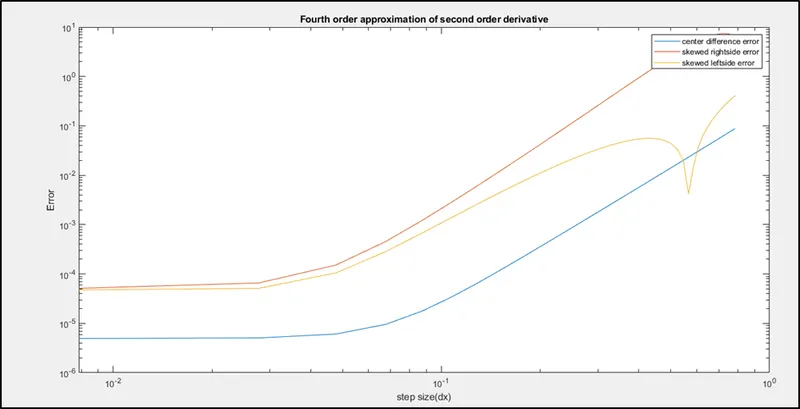
5. Plot the graph between stepsize(dx) and the different error involves in different approximation method.

• OUTPUT PLOT:

• CONCLUSION:
• From the above plot it is clear that 4th order approximation of 2nd order derivative using Center difference method gives less error when compared to the other two scheme.
• If we want to compute approximation for a function at a boundary or last node,we cannot use center difference scheme at this particular node as this method uses past and future data to calculate the data at present point,in this senario skewed difference scheme plays a vital role and allow us to compute the approximation at the boundary.