Deriving 4th order approximation of a 2nd order derivative using Taylor Table method
AIM:
To derive the fourth order approximation of a second order derivative using central differencing scheme,skewed right difference scheme and skewed left difference scheme with the help of Taylor table and also to compare the obtained values with analytical derivative value for the given function.
OBJECTIVE:
- After deriving these schemes,To prove that the skewed schemes are fourth-order accurate i.e the thumb rule given in HINT (ii).
- To write a program in Matlab to evaluate the second-order derivative of the analytical function exp(x)*cos(x) and compare it with the 3 numerical approximations that after derived.
- To Provide a plot that compares the absolute error between the above-mentioned schemes
HINT :
i) The order of accuracy P = Number of nodes in the stencil N - order of derivative Q + 1 for symmetric/central schemes
ii) The order of accuracy P = Number of nodes in the stencil N - order of derivative Q for one-sided/skewed schemes
iii) Solve the system of equations using the matrix inversion method in Matlab to obtain the taylor table coefficients and use them directly in the numerical approximation statements to avoid input errors.
THEORY:
1.Fourth order approximation of a second order derivative using central differencing scheme:
Numerical stencil for central differencing scheme
Let us consider the approximation
∂2u∂x2≈af(i-2)+bf(i-1)+cf(i)+df(i+1)+ef(i+2)dx2+O(dx4)">∂2u∂x2≈af(i−2)+bf(i−1)+cf(i)+df(i+1)+ef(i+2)dx2+O(dx4) ---------equation (1)
af(i-2)=af(i)-af′(i)⋅(2dx)1!+af′′(i)⋅(2dx)22!-af′′′(i).(2dx)33!+af′′′′(i).(2dx)44!-----">af(i−2)=af(i)−af'(i)⋅(2dx)1!+af''(i)⋅(2dx)22!−af'''(i).(2dx)33!+af''''(i).(2dx)44!
expand the above terms till fourth order
similarly expand all the terms present in eq (1). Now these terms are represented in the form of a table to solve for the coefficients of eq (1) and this can be solved using Taylor Table Method.
|
stencil/taylor series terms |
f(i)">f(i) |
dx⋅f′(i)">dx⋅f'(i) |
dx2⋅f′′(i)">dx2⋅f''(i) |
dx3⋅f′′′(i)">dx3⋅f'''(i) |
dx4⋅f′′′′(i)">dx4⋅f''''(i) |
|
af(i-2) |
a |
-2a |
4a/2 |
-8a/6 |
16a/24 |
|
bf(i-1) |
b |
-b |
b/2 |
-b/6 |
b/24 |
|
cf(i) |
c |
0 |
0 |
0 |
0 |
|
df(i+1) |
d |
d |
d/2 |
d/6 |
d/24 |
|
ef(i+2) |
e |
2e |
4e/2 |
8e/6 |
16e/24 |
|
sum of the coefficients |
0 |
0 |
1 |
0 |
0 |
From the above table when we sum the derivative terms we get the following set of equations
a+b+c+d+e=0">a+b+c+d+e=0a+b+c+d+e=0
-2a-b+0+d+2e=0">−2a−b+0+d+2e=0-2a-b+0+d+2e=0
2a+b2+0+d2+2e=1">2a+b2+0+d2+2e=12a+b2+0+d2+2e=1
-8a6-b6+0+d6+8e6=0">−8a6−b6+0+d6+8e6=0-8a6-b6+0+d6+8e6=0
16a24+b24+0+d24+16e24=0">16a24+b24+0+d24+16e24=016a24+b24+0+d24+16e24=0
the above set of linear equations have to be solved using matrix inversion method and hence are to be represented in the form of matrix i.e.
AX = B
from the above values we have a = -0.0833, b = 1.3333, c = -2.5000, d = 1.3333, e = -0.0833
substituting in eq (1) yields to our approximation
(∂2u∂x2)≈(-0.0833)(f(i-2))+(1.3333)(f(i-1))+(-2.5000)(f(i))+(1.3333)(f(i+1))+(-0.0833)(f(i+2))dx2+O(dx4)">(∂2u∂x2)≈(−0.0833)(f(i−2))+(1.3333)(f(i−1))+(−2.5000)(f(i))+(1.3333)(f(i+1))+(−0.0833)(f(i+2))dx2+O(dx4)
2.Fourth order approximation using skewed right difference scheme:
Numerical stencil for skewed diiference scheme
Let us consider the approximation
∂2u∂x2≈af(i)+bf(i+1)+cf(i+2)+df(i+3)+ef(i+4)dx2+O(dx4)">∂2u∂x2≈af(i)+bf(i+1)+cf(i+2)+df(i+3)+ef(i+4)dx2+O(dx4)
expanding each of the terms and putting them in the taylor table then we have our table as shown below:
|
stencil/taylor series terms |
f(i)">f(i) |
dx⋅f′(i)">dx⋅f'(i) |
dx2⋅f′′(i)">dx2⋅f''(i) |
dx3⋅f′′′(i)">dx3⋅f'''(i) |
dx4⋅f′′′′(i)">dx4⋅f''''(i) |
|
af(i) |
a |
0 |
0 |
0 |
0 |
|
bf(i+1) |
b |
b |
b/2 |
b/6 |
b/24 |
|
cf(i+2) |
c |
2c |
4c/2 |
8c/6 |
16c/24 |
|
df(i+3) |
d |
3d |
9d/2 |
27d/6 |
81d/24 |
|
ef(i+4) |
e |
4e |
16e/2 |
64e/6 |
256e/24 |
|
sum of coefficients |
0 |
0 |
1 |
0 |
0 |
adding the derivative terms we get the equations as:
a+b+c+d+e=0">a+b+c+d+e=0a+b+c+d+e=0
0+b+2c+3d+4e=0">0+b+2c+3d+4e=00+b+2c+3d+4e=0
0+b2+2c+92d+8e=1">0+b2+2c+92d+8e=10+b2+2c+92d+8e=1
0+b6+86c+276d+646e=0">0+b6+86c+276d+646e=00+b6+86c+276d+646e=0
0+b24+1624c+8124d+25624e=0">0+b24+1624c+8124d+25624e=00+b24+1624c+8124d+25624e=0
the above set of linear equations have to be solved using matrix inversion method and hence are to be represented in the form of matrix i.e.
AX = B
from the above we have a=2.9167, b = -8.6667, c = 9.5000, d = -4.6667, e = 0.9167. Substituting these values in eq (2) we have our approximation
∂2u∂x2≈2.9167f(i)-8.6667f(i+1)+9.5000f(i+2)-4.6667f(i+3)+0.9167f(i+4)dx2+O(dx4)">∂2u∂x2≈2.9167f(i)−8.6667f(i+1)+9.5000f(i+2)−4.6667f(i+3)+0.9167f(i+4)dx2+O(dx4)
3.Fourth order approximation using skewed left difference scheme:
Numerical stencil for skewed left differencing scheme
Let us consider the approximation
∂2u∂x2≈af(i-4)+bf(i-3)+cf(i-2)+df(i-1)+ef(i)dx2+O(dx4)">∂2u∂x2≈af(i−4)+bf(i−3)+cf(i−2)+df(i−1)+ef(i)dx2+O(dx4) -------equation (3)
expanding each of the terms and putting them in the taylor table then we have our table as shown below:
|
stencil/taylor series terms |
f(i)">f(i) |
dx⋅f′(i)">dx⋅f'(i) |
dx2⋅f′′(i)">dx2⋅f''(i) |
dx3⋅f′′′(i)">dx3⋅f'''(i) |
dx4⋅f′′′′(i)">dx4⋅f''''(i) |
|
af(i-4) |
a |
-4a |
8a |
-64a/6 |
-256a/24 |
|
bf(i-3) |
b |
-3b |
9b/2 |
-27b/6 |
81b/24 |
|
cf(i-2) |
c |
-2c |
2c |
-8c/6 |
16c/24 |
|
df(i-1) |
d |
-d |
d/2 |
-d/6 |
d/24 |
|
ef(i) |
e |
0 |
0 |
0 |
0 |
|
sum of coefficients |
0 |
0 |
1 |
0 |
0 |
adding the derivative terms we get the equations as:
a+b+c+d+e=0">a+b+c+d+e=0a+b+c+d+e=0
-4a-3b-2c-d+0=0">−4a−3b−2c−d+0=0-4a-3b-2c-d+0=0
8a+92b+2c+d2+0=0">8a+92b+2c+d2+0=08a+92b+2c+d2+0=0
-646a-276b-86c-d6+0=0">−646a−276b−86c−d6+0=0-646a-276b-86c-d6+0=0
25624a+8124b+1624c+d24+0=0">25624a+8124b+1624c+d24+0=025624a+8124b+1624c+d24+0=0
the above set of linear equations have to be solved using matrix inversion method and hence are to be represented in the form of matrix i.e.
AX = B
from the above we have a=0.9167, b = -4.6667, c = 9.5000, d = -8.6667, e = 2.9167. Substituting these values in eq (3) we have our approximation
∂2u∂x2≈0.9167f(i-4)-4.6667f(i-3)+9.5000f(i-2)-4.6667f(i-1)+0.9167f(i)dx2+O(dx4)">∂2u∂x2≈0.9167f(i−4)−4.6667f(i−3)+9.5000f(i−2)−4.6667f(i−1)+0.9167f(i)dx2+O(dx4)
4. Approximation using Forward differencing scheme:
The approximation for forward differencing scheme is
d2f(x)dx2=2f(x+a)-f(x)-f′(x)⋅dxdx2">d2f(x)dx2=2f(x+a)−f(x)−f'(x)⋅dxdx2
5. Approximation using Backward differencing scheme:
The approximation for backward differencing scheme is
d2f(x)dx2=2f(x-a)-f(x)+f′(x)⋅dxdx2">d2f(x)dx2=2f(x−a)−f(x)+f'(x)⋅dxdx2
MATLAB CODE:
- d2f(x)dx2=2f(x-a)-f(x)+f′(x)⋅dxdx2">Defining the function for central differencing scheme
function error_central_diff = central_difference(x,dx)

 % f(x) = e^(x)*cosx is the given function

 % second order derivative for the given function

   second_analytical_derivative = -2*exp(x)*sin(x);

    % calculating the central differencing value

    central_differencing = (((-0.0833)*((exp(x-(2*dx)))*(cos(x-(2*dx)))))+((1.3333)*((exp(x-dx))*(cos(x-dx))))-((2.5)*((exp(x))*(cos(x))))+((1.3333)*((exp(x+dx))*(cos(x+dx))))+((-0.0833)*((exp(x+(2*dx)))*(cos(x+(2*dx))))))/(dx^2);

    % calculating the absolute error

    error_central_diff = abs(central_differencing - second_analytical_derivative)
end
- Defining the function for skewed right differencing scheme
function error_skewed_right = skewed_right_difference(x,dx)

 % f(x) = e^(x)*cosx is the given function

 % second order derivative for the given function

 second_analytical_derivative = -2*exp(x)*sin(x);

 % Calculating the skewed right differencing value

    skewed_right_diff = (((2.9167)*((exp(x))*(cos(x))))-((8.6667)*((exp(x+dx))*(cos(x+dx))))+((9.5000)*((exp(x+(2*dx))*(cos(x+(2*dx))))))-((4.6667)*((exp(x+(3*dx)))*(cos(x+(3*dx)))))+((0.9167)*((exp(x+(4*dx)))*(cos(x+(4*dx))))))/(dx^2);

    % Calculating the absolute error

    error_skewed_right = abs(skewed_right_diff-second_analytical_derivative)
end- Defining the function for skewed left differencing scheme
function error_skewed_left = skewed_left_difference(x,dx)

% f(x) = e^(x)*cosx is the given function

 % second order derivative for the given function

   second_analytical_derivative = -2*exp(x)*sin(x);

    % Calculating the skewed right differencing value

    skewed_left_diff = (((0.9167)*((exp(x-(4*dx))*(cos(x-(4*dx))))))-((4.6667)*((exp(x-(3*dx))*(cos(x-(3*dx))))))+((9.5000)*((exp(x-(2*dx))*(cos(x-(2*dx))))))-((8.6667)*((exp(x-dx))*(cos(x-dx))))+((2.9167)*((exp(x))*(cos(x)))))/(dx^2);

    % Calculating the absolute error

    error_skewed_left = abs(skewed_left_diff-second_analytical_derivative)
end
- Defining the function for forward differencing scheme
function error_forward_diff = forward_difference(x,dx)

% f(x) = e^(x)*cosx is the given function

% first_analytical_derivative = exp(x)*(cos(x)-sin(x))

 % second order derivative for the given function

   second_analytical_derivative = -2*exp(x)*sin(x);

    % calculating the forward differencing value

   forward_differencing = (2*((exp(x+dx)*cos(x+dx))-(exp(x)*cos(x))-((exp(x)*(cos(x)-sin(x)))*dx)))/(dx^2);

    % calculating the absolute error

   error_forward_diff = abs(forward_differencing - second_analytical_derivative)
end- Defining the function for backward differencing scheme
function error_backward_diff = backward_difference(x,dx)

% f(x) = e^(x)*cosx is the given function

% first_analytical_derivative = exp(x)*(cos(x)-sin(x))

 % second order derivative for the given function

   second_analytical_derivative = -2*exp(x)*sin(x);

   % calculating the backward differencing value

   backward_differencing = (2*((exp(x-dx)*cos(x-dx))-(exp(x)*cos(x))+((exp(x)*(cos(x)-sin(x)))*dx)))/(dx^2);

   % calculating the absolute error

   error_backward_diff = abs(backward_differencing - second_analytical_derivative)

end
MAIN CODE:
STEP WISE EXPLANATION:
clear all
close all
clc

% Declaring the value for 'x'

x = pi/3;

% Declaring the variable 'dx'

dx = linspace(pi/4,pi/40,10);
- Start with clear all close all clc
- Here the x and dx variables are declared and stored
% To begin a for loop to calculate the values of different schemes

for i = 1:length(dx)   % declaring the variable 'i'

    central_diff_value(i) = central_difference(x,dx(i));  % Calling the function central difference

    skewed_right_value(i) = skewed_right_difference(x,dx(i));  % Calling the function skewed right difference

    skewed_left_value(i) = skewed_left_difference(x,dx(i));     % Calling the function skewed left difference

    forward_diff_value(i) = forward_difference(x,dx(i));        % Calling the function forward difference

    backward_diff_value(i) = backward_difference(x,dx(i));       % Calling the function backward difference

end- For loop is used to caluculate the values for different schemes from central to backward difference
figure(1)

loglog(dx,central_diff_value,'r','linewidth',3)
hold on
loglog(dx,skewed_right_value,'b','linewidth',3)
hold on
loglog(dx,skewed_left_value,'c','linewidth',3)
hold on
loglog(dx,forward_diff_value,'g','linewidth',3)
hold on
loglog(dx,backward_diff_value,'y','linewidth',3)

xlabel('dx','FontSize',20)
ylabel('error','FontSize',20)

legend('CENTRAL DIFF ERROR','SKEWED RIGHT ERROR','SKEWED LEFT ERROR','FORWARD DIFF ERROR','BACKWARD DIFF ERROR')
- Graph is plotted using log log plot for different schemes with dx
- providing each of them with different colours and labels are given
- legend is stored with the all schemes respectively.
FINAL CODE:
clear all
close all
clc

% Declaring the value for 'x'

x = pi/3;

% Declaring the variable 'dx'

dx = linspace(pi/4,pi/40,10);

% To begin a for loop to calculate the values of different schemes

for i = 1:length(dx)   % declaring the variable 'i'

    central_diff_value(i) = central_difference(x,dx(i));  % Calling the function central difference

    skewed_right_value(i) = skewed_right_difference(x,dx(i));  % Calling the function skewed right difference

    skewed_left_value(i) = skewed_left_difference(x,dx(i));     % Calling the function skewed left difference

    forward_diff_value(i) = forward_difference(x,dx(i));        % Calling the function forward difference

    backward_diff_value(i) = backward_difference(x,dx(i));       % Calling the function backward difference

end


% Plotting the graph using log-log plot

figure(1)

loglog(dx,central_diff_value,'r','linewidth',3)
hold on
loglog(dx,skewed_right_value,'b','linewidth',3)
hold on
loglog(dx,skewed_left_value,'c','linewidth',3)
hold on
loglog(dx,forward_diff_value,'g','linewidth',3)
hold on
loglog(dx,backward_diff_value,'y','linewidth',3)

xlabel('dx','FontSize',20)
ylabel('error','FontSize',20)

legend('CENTRAL DIFF ERROR','SKEWED RIGHT ERROR','SKEWED LEFT ERROR','FORWARD DIFF ERROR','BACKWARD DIFF ERROR')
OUTPUT:
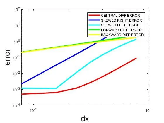
RESULTS:
- From the above plots we can say that Central differencing scheme gives the least error value when comapred to other differencing schemes. Central differencing scheme utilises the information available at next neighbouring points on both the sides from the point of consideration to give the approximation value. CDS results in giving higher order approximations and we know that as order of approximation increases the error decreases. The advantage of CDS is that its convergence rate is faster than all other differencing schemes.
- Next scheme after CDS is Skewed Left Differencing Scheme and then comes Skewed Right Differencing Scheme in the context of least errors. Though initially Skewed Right Differencing Scheme is resulting in highest errors as per the plot but as 'dx' value decreases it stands next to Skewed Left Differencing Scheme. Skewed differencing schemes utilises the information available at next neighbouring points on one side from the point of consideration either left or right to give the approximation value. This scheme is used in computing higher order approximations. When compared with CDS, the error obtained with skewed schemes are relatively high.
- Backward differencing and Forward differencing are next in the hierarchy of errors.These are used to compute the first order approximations. These schemes use the information available at next neighbouring point on one side from the point of consideration to give the approximation value and hence the error obtained with these schemes are relatively high.