Week 3.4 - Discretization for range of dx

QUESTION:

In part 1, you had computed the first, second, and fourth-order approximations for a given value of x and dx.

For this program, you need to do the following.

1. For a range of dx, plot the first order, second and fourth-order error.

dx range = [pi/4000,pi/40,20]

2. Make sure that you plot dx vs error in a way that makes sense.
3. Explain the results in the space provided. What can you say about the slope of the curves in this plot?
4. Write a detailed explanation for your results, plots or codes without explanation will be awarded zero marks.

ANSWER:

AIM:

• To compute the first, second, and fourth-order errors for the first derivative of the function and compare them with respect to grid spacing(dx).
• To calculate the slope of the curves and discuss the significance.

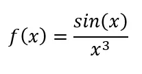
FUNCTION:

Function –

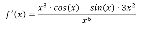
First Derivative of the function –

X = pi/3, dx = linspace(pi/4000,pi/40,20)

INPUT: -

[MATLAB CODE]

%% Initialization
clc
close all
clear all

%% Function to be Discritized
% f(x) = sin(x)/x^3

%% Stencil Values
x = pi/3;
dx = linspace(pi/4000,pi/40,20);

%% Annalytical Discritization

annalytical_value = ((x^3)*(cos(x)) - (sin(x))*3*(x^2))/(x^6);

%% First Order Approximation

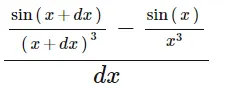
first_order_approx = ((sin(x+dx))./((x+dx)).^3 - (sin(x))./(x^3))./dx;

%% Second-Order Approximation

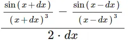
second_order_approx = ((sin(x+dx)./(x+dx).^3) - (sin(x-dx)./(x-dx).^3))./(2*dx);

%% Fourth Order Approximation

fourth_order_approx = (sin(x-2*dx)./(x-2*dx).^3 - 8*(sin(x-dx)./(x-dx).^3) + 8*(sin(x+dx)./(x+dx).^3) - (sin(x+2*dx)./(x+2*dx).^3))./(12*dx);

%% Error calculation

first_order_error = abs(first_order_approx - annalytical_value);
second_order_error = abs(second_order_approx - annalytical_value);
fourth_order_error = abs(fourth_order_approx - annalytical_value);
error = [first_order_error, second_order_error, fourth_order_error];

%% Graph plotting

loglog(dx,first_order_error,'linewidth',3);
hold on
loglog(dx,second_order_error,'linewidth',3);
loglog(dx,fourth_order_error,'linewidth',3);
xlabel('dx');
ylabel('ERROR');
legend('First Order','Second Order','Fourth Order')
grid on

%% Slope Calculation
% Calculating the absolute error and dx in terms of log10

first_error_log = log10(first_order_error);
second_error_log = log10(second_order_error);
fourth_error_log = log10(fourth_order_error);
dx_log = log10(dx);

% To calculate the slope
slope_1 = diff(first_error_log)./diff(dx_log);
slope_2 = diff(second_error_log)./diff(dx_log);
slope_3 = diff(fourth_error_log)./diff(dx_log);

EXPLINATION: -

• As we can see here, first the analytical derivative is calculated at
• X and dx values are assigned. For the dx value, the ‘linspace’ command is used to define the range of dx.
• In the function the analytical derivative value is,

• For first-order approximation, forward differencing is used,

• For second-order approximation, central differencing is used,

• For fourth-order approximation, central differencing is used,

• The error value for each is calculated by taking the difference between the respective order of differencing and the analytical derivative value.
• Thus, for each value of dx, the above steps are repeated and the error is calculated.
• Now for plotting instead of using plot command, loglog command is used. This command is used if the graphs are exponential and difficult to compare.
• So, using loglog plots, the curves are converted to straight lines and become easy to compare. Grid spacing(dx) taken along X-axis, and absolute error taken along Y-axis.
• The xlabel, ylabel, and Legend are given.
• The next step is to find the slope of the curve, since it is a loglog plot, the absolute error and grid spacing (dx) is converted in terms of log(base10) and storing values to another variable.
• Slope between any two point is calculated as, slope = difference in absolute error(in log10)/difference in grid spacing(dx).

OUTPUT:

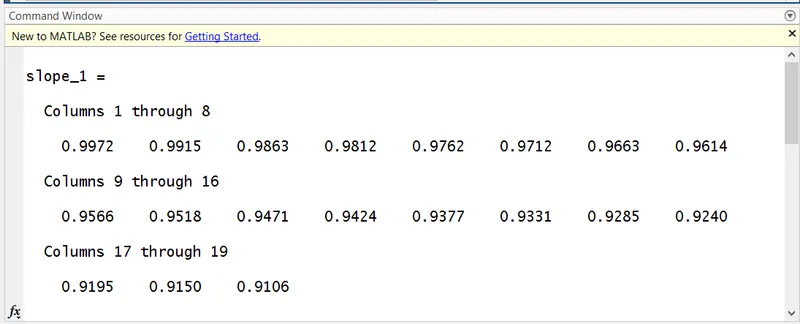
The slope of first-order error:

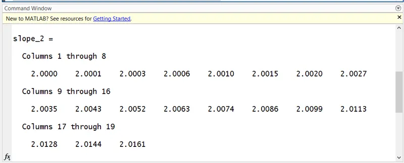
The slope of second-order error:

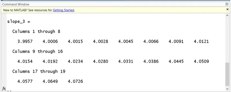
The slope of fourth-order error:

Graph:

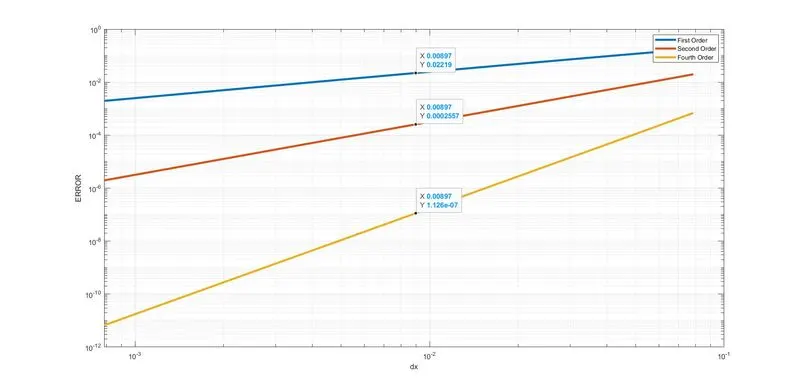
Hence, from the above-obtained graph, we can see conclude that,

First-order error > Second-order error > Fourth-order error

Significance of Slope:

• The slope for the three plots is positive since the line moves upward when moving from left to right.
• Slope also tells us the rate at which change takes place.
• For first-order error, slope = 0.9 when moving from left to right (when dx increases), rate of increase of absolute error is least.
• For fourth-order error, slope = 4.0 when moving from left to right (when dx increases), the rate of increase of absolute error is highest.
• For second-order error, slope = 2 the rate of increase of absolute error is greater than the first-order error but less than the fourth-order error.

CONCLUSION:

• Thus, the first, second, and fourth-order error for the first derivative of a function is computed and compared with respect to the change in grid spacing (dx).
• The slope is calculated for each absolute error and their significance is explained clearly.