Week 3.2 - 2R Robotic Arm Challenge
Forward Kinematics of a Robotic arm
Aim:
To simulate the forward kinematics of a 2R robotic arm to visualize its end-effector trajectory as the joint angles change.
Explanation:
The aim of this program is to simulate the forward kinematics of a 2R
robotic arm, a functional concept in robotics. Forward kinematics involves
determing the position and orientation of the robot’s end-effector (in this
case, the “hand” of the robotic arm) based on the angles of its joints.
Initilazation:
<!--[if !supportLists]-->o
<!--[endif]-->We start by defining the physical parameters
of the robotic arm, such as the lengths of its links and the range of joint
angles we want to explore.
Looping Through Joint Angles:
<!--[if !supportLists]-->o
<!--[endif]-->We use nested loops to iterate through
different joint angle combinations, allowing us to explore how the arm’s
configuration affects its effect-effector’s position.
Forward Kinematics Calculations:
<!--[if !supportLists]-->o
<!--[endif]-->Within the loops, we calculate the position of
the end-effector using forward kinematics equations, which take into account
the lengths of the links and the joint angles. These equations involve trigonometric
functions to determine the coordinates (x,y) of the end-effector.
Visualization:
<!--[if !supportLists]-->o
<!--[endif]-->We visualize the robotic arm’s configuration
and the path of the end-effector by plotting its trajectory. This helps us gain
insights into how the arm moves in
response to changes in joint angles.
Animation (Optional):
<!--[if !supportLists]-->o
<!--[endif]-->If desired, we can recreate an animation to
observe the arm’s motion as it moves through various joint configurations. This
can be useful for educational purposes or for better understanding the robot’s
behavior.
Display or save Results:
<!--[if !supportLists]-->o
<!--[endif]-->Finally, we can display the reulsts on the
screen or save them to a file (e.g., for creating videos or reports) to analyze
and present the simulated robotic arm’s behavior.
Solved Errors :
ERROR 1: (Case Sensitive)
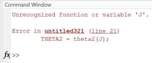
In MATLAB, variable names are case-sensitive. The uppercase ‘J’ is used instead of lowercase ‘j’ .
<!--[if !supportLists]-->· <!--[endif]-->Line No. 21
Line with Error: THETA2 = theta(J);
Correction: Change ‘J’ to ‘j’ to correctly reference the loop variable.
ERROR 2: (Typo in ‘sin’ Function)
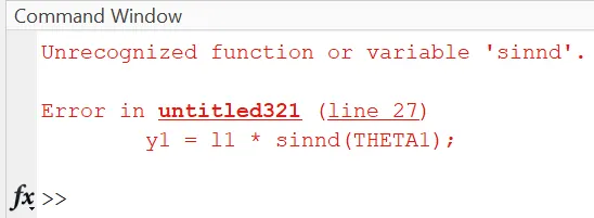
There is a typo in the ‘sin’ function, but have used ‘sinnd’ instead of ‘sind’ for calculating the sine of ‘THETA2’.
<!--[if !supportLists]-->· <!--[endif]-->Line No. 27
Line with
Error: y2 = y1 + l2 * sinnd(THETA2);
Correction:
Replace ‘sinnd’ with ‘sind’ to calculate the sine correctly.
y2 = y1 + l2 * sind(THETA2);
ERROR 3: (Plotting Function Error)
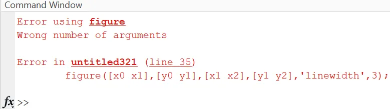
The ‘figure’ function is used to create
a new figure window, but you intended to use the ‘plot’ function to create the plot.
<!--[if !supportLists]-->·
<!--[endif]-->Line No.35
Line with Error: ‘figure’ ([x0 x1], [y0 y1],
[x1 x2], [y1 y2], ‘linewidth’, 3);
Correction: Replace ‘figure’ with ‘plot’ and
adjust the syntax for plotting.
ERROR 4: ( Syntax Error in ‘axis’ Function)

There is a syntax error in the ‘axis’ function. The closing
paranthesis is missing.
<!--[if !supportLists]-->· <!--[endif]-->Line No. 36
Line with Error: axis([-0.1 1.5 0 1.5]
Correction: Add a closing paranthesis to the ‘axis’ function
to fix the syntax error: axis([-0.1 1.5 0 1.5)]
ERROR 5: ( Undefined Variable Error)
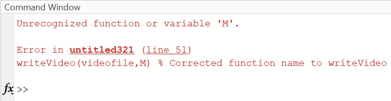
The
variable ‘M’ is used to store frames for the animation, but it’s not
initialized before use.
<!--[if !supportLists]-->· <!--[endif]-->Line No. 38,46& 51
Line with Error: m(ct) = getframe(gcf); and
movie(m);
movie(m)
writeVideo(videofile,m)
Correction: Initialize ‘M’ as an empty array before
the loop.
M(ct) = getframe(gcf); and movie(M)
writeVideo(videofile,M)
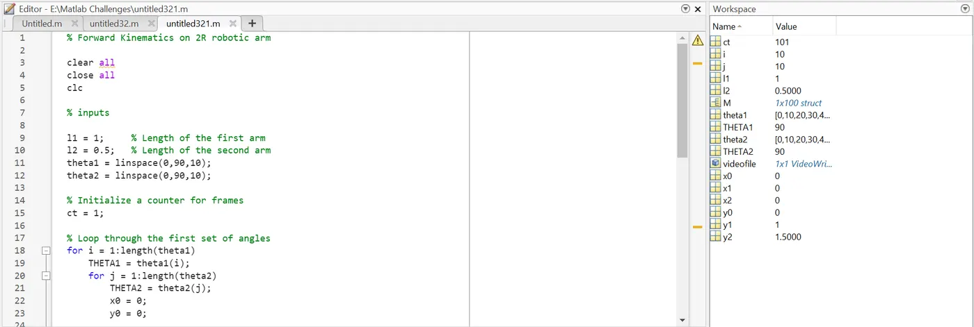
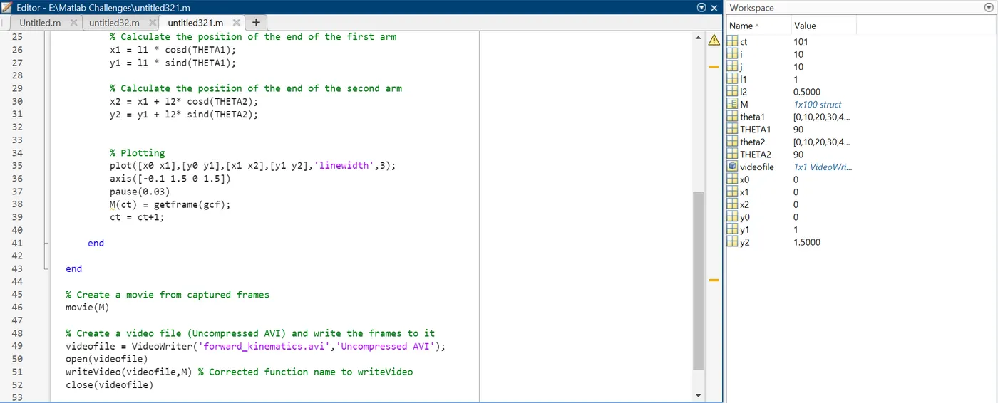
Code with comments:
% Forward Kinematics on 2R
robotic arm
clear all
close all
clc
% inputs
l1 = 1; % Length of the first arm
l2 = 0.5; % Length of the second arm
theta1 = linspace(0,90,10); ( Range of angles for
the first joint (0 to 90degrees)
theta2 = linspace(0,90,10); ( Range of angles for
the second joint (0 to 90 degrees)
% Initialize a counter for
frames
ct = 1;
% Loop through the first set of
angles
for i = 1:length(theta1)
THETA1 =
theta1(i);
for j = 1:length(theta2)
THETA2 = theta2(j);
x0 =
0;
y0 =
0;
�lculate the position of the end of the first arm
x1 =
l1 * cosd(THETA1);
y1 =
l1 * sind(THETA1);
�lculate the position of the end of the second arm
x2 =
x1 + l2* cosd(THETA2);
y2 =
y1 + l2* sind(THETA2);
% Plotting
plot([x0 x1],[y0 y1],[x1 x2],[y1 y2],'linewidth',3);
axis([-0.1 1.5 0 1.5])
pause(0.03)
M(ct)
= getframe(gcf); (Capture the current
frame)
ct =
ct+1; (Increment the frame
counter)
end
end
% Create a movie from captured
frames
movie(M)
% Create a video file
(Uncompressed AVI) and write the frames to it
videofile = VideoWriter('forward_kinematics.avi','Uncompressed AVI');
open(videofile)
writeVideo(videofile,M) %
Corrected function name to writeVideo
close(videofile)
Expalnation of Code:
% inputs
l1 = 1; % Length of the first arm
l2 = 0.5; % Length of the second arm
These lines defines the lengths of the two robotic arms (‘l1’ and
‘l2’).
theta1 = linspace(0,90,10);
theta2 = linspace(0,90,10);
Here, you generate two sets of angles (‘theta1’ and
‘theta2’) using ‘linspace’. These angles define the range of motion
for the two joints of the robotic arm
% Initialize a counter for
frames
ct = 1;
These lines initializes a counter variable ‘ct’ to
keep of frames for creating the animation
% Loop through the first set of
angles
for i = 1:length(theta1)
THETA1 =
theta1(i);
for j = 1:length(theta2)
THETA2 = theta2(j);
x0 =
0;
y0 =
0;
These lines start nested loops to iterate through each combination of ‘theta1’
and ‘theta2’ values. Inside
these loops, you set the current values of ‘THETA1’ and ‘THETA2’ and
initialize ‘x0’ and ‘y0’ for the starting point of the robotic
arm.
�lculate the position of the
end of the first arm
x1 =
l1 * cosd(THETA1);
y1 =
l1 * sind(THETA1);
These lines calculates
the position (‘x1’, ‘y1’) of the end of the first arm using
trigonometric functions (‘cosd’ for cosine and ‘sind’ for shine)
to convert the joint angles into Cartesian coordinates.
�lculate the position of the
end of the second arm
x2 =
x1 + l2* cosd(THETA2);
y2 =
y1 + l2* sind(THETA2);
Simarly, these lines calculates the position (‘x2’, ‘y2’) of the
end of the second arm by adding ‘l2’ times the cosine and shine of ‘THETA2’
to the coordinates of the first arm’s end.
% Plotting
plot([x0
x1],[y0 y1],[x1 x2],[y1 y2],'linewidth',3);
axis([-0.1
1.5 0 1.5])
pause(0.03)
M(ct) =
getframe(gcf);
ct = ct+1;
Here, you plot the robotic arm by drawing lines connecting the points ‘[x0
y0]’ to ‘[x1 y1]’ and ‘[x1 y1]’ to ‘[x2 y2]’. The ‘plot’
function also specifies the line width. The ‘axis’ function sets the
axis limit fro the plot. ‘pause(0.03)’ add a short delay to control the
frame rate. ‘getframe(gcf)’ captures the current frame, and it is stored
in the ‘M’ array. The ‘ct’ counter is incremented to keep track
of frames.
end
end
These lines close the nested loops, completing the animation frames for
all combinations of joint angles.
% Create a movie from captured
frames
movie(M)
These lines creates a movie from the captured frames stored in the ‘M’
array.
% Create a video file
(Uncompressed AVI) and write the frames to it
videofile = VideoWriter('forward_kinematics.avi','Uncompressed AVI');
open(videofile)
writeVideo(videofile,M) %
Corrected function name to writeVideo
close(videofile)
These lines creates a video file named ‘forward_kinematics.avi’ in
‘Uncompressed AVI’ format, open the file for writing, and write the
frames from the ‘M’ array to the video file. Finally, the video file is
closed.
This code simulates the forward kinematics of a 2R robotic arm and
generates an animation of its motion as the joint angles vary.
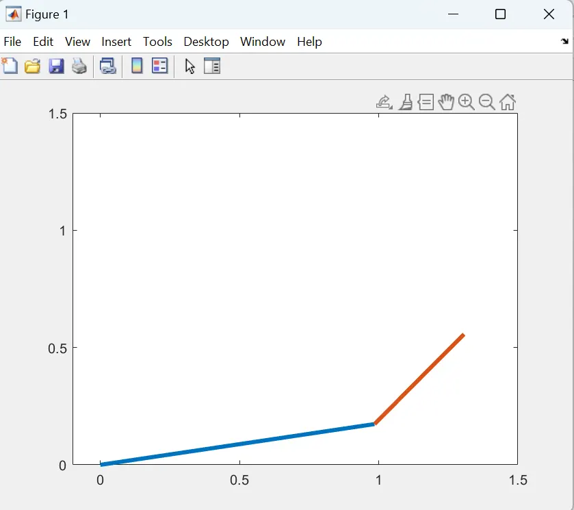
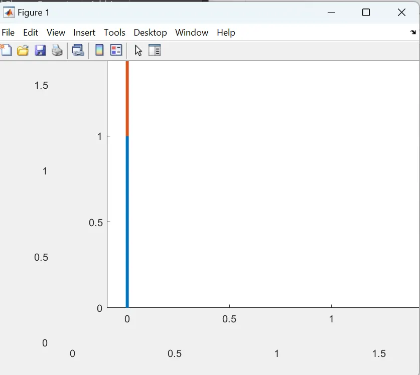
Explanation of Output:
The output of the provided MATLAB program is an animation that
visualizes the forward kinematics of a 2R robotic arm. Let’s break down the
output and what it represents.
1. Animation:
<!--[if !supportLists]-->·
<!--[endif]-->The main output is an animation that shows the
movement of the 2R robotic arm as it changes its joint angles. The animation
displays the arm’s configurations of ‘theta1’ and ‘theta2’.
2.
Graphical Representation:
<!--[if !supportLists]-->·
<!--[endif]-->In the animation, you see a graphical
representation of this robotic arm composed of two segements.
<!--[if !supportLists]-->o
<!--[endif]-->Link1:
The first
arm link (l1) is typically represented by a line segement that extends
from the base (starting point) to its end point. The length of this link is
defined by the ‘l1’ parameter.
<!--[if !supportLists]-->o
<!--[endif]-->Link2:
The second arm link (l2) is similarly represented by a line segment
extending from the end point of Link 1 to its own end
point. The length of this link is defined by the ‘l2’ parameter.
3. Joint Movement:
<!--[if !supportLists]-->·
<!--[endif]-->As the animation progresses, you observe that the joint angles (‘theta1’ and ‘theta2’) change. These
changes in joint angles correspond to the motion of the robotic arm. The arm’s
movement demonstrates how different combinations of joint angles result in
various positions of the end effector ( the tip of Link 2).
4. Iteration through joint
Angles:
<!--[if !supportLists]-->·
<!--[endif]-->The animation is created by systematically
iterating through different combinations of ‘theta1’ and ‘theta2’. For each combination, the
program calculates the positions of the end points of Link 1 and Link 2, and
then plots these positions to represent the arm’s configuration.
5. Real-Time Visulaization:
<!--[if !supportLists]-->·
<!--[endif]-->The animation is generated frame by frame, and
each frame corresponds to a specific set of joints angles. The animation runs
in real-time, showing the continuous movement of the robotic arm.
6. Video File:
<!--[if !supportLists]-->·
<!--[endif]-->The program also saves this animation as an
uncompressed AVI video file named ‘froward_kinematics.avi’. This video
file can be played back to review the motion of the 2R robotic arm or shared
with others for educational or explanatory purposes.
OUTPUT:
https://drive.google.com/file/d/1eFgMyqXI1EZZCWmFtPJlvS5a_DOgBF1e/view?usp=sharing