Week 2 Railwheel and Track
WEEK 2 : RAILWHEEL AND TRACK
1. Objective
a) To perform a static structural analysis on the Railwheel and Track setup with a bearing load of 100000 N and
500000 N and compare the equivalent stress, life and total deformation.
b) To compare the total deformation results given by ANSYS and that obtained from user defined result.
2. Case Setup and Execution
The assembly provided for analysis consists of a railwheel, track and bearing as shown in Figure 1. The material assigned to all the parts is structural steel.
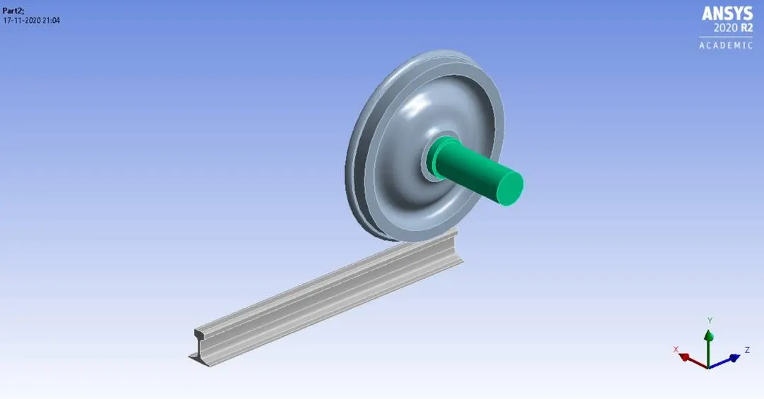
Fig 1. Railwheel Track Assembly
2.a Mesh
The global mesh size used for the assembly is 50 mm while face sizing with mesh size of 35 mm is used at the contact face of railwheel and track as this area will be subjected to maximum stress after the application of load. The mesh is shown in Figure 2.
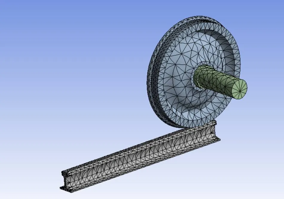
Fig 2. Mesh Generation with Face Sizing
2.b Contact Setup
For the railwheel and track, a frictional contact with a coefficient of friction value of 0.3 is assigned while frictionless contact is assigned between railwheel and bearing.
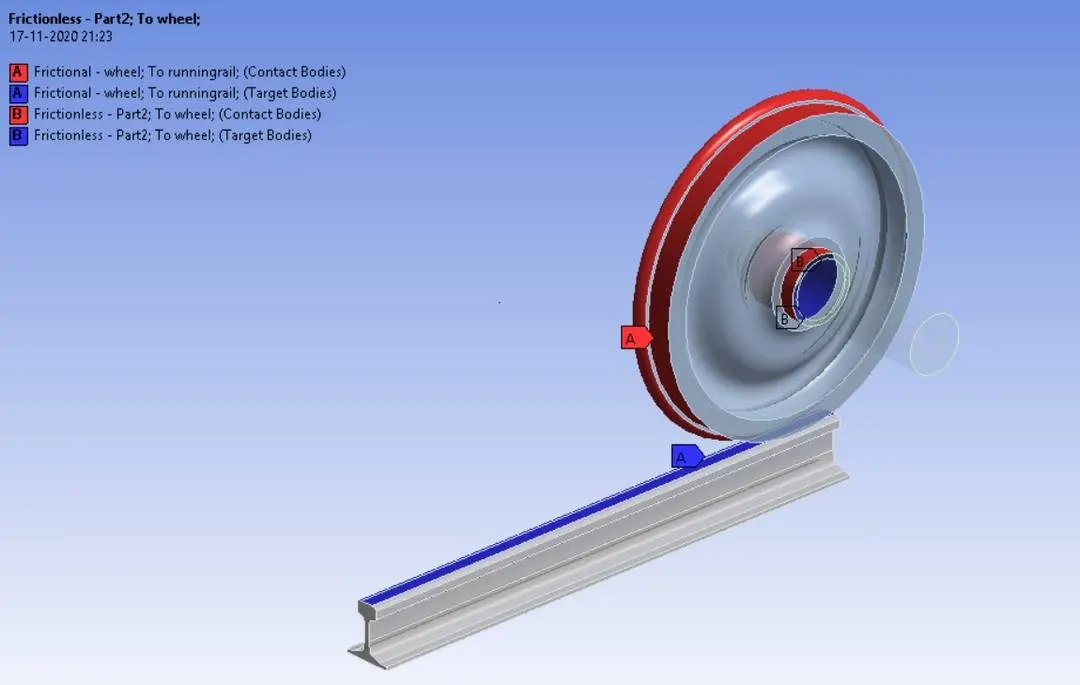
Fig 3. Contact Definition between mating pairs
2.c Boundary Conditions
The two faces of the track are fixed as shown in Figure 4. The connection type is Body-Ground and type - fixed.
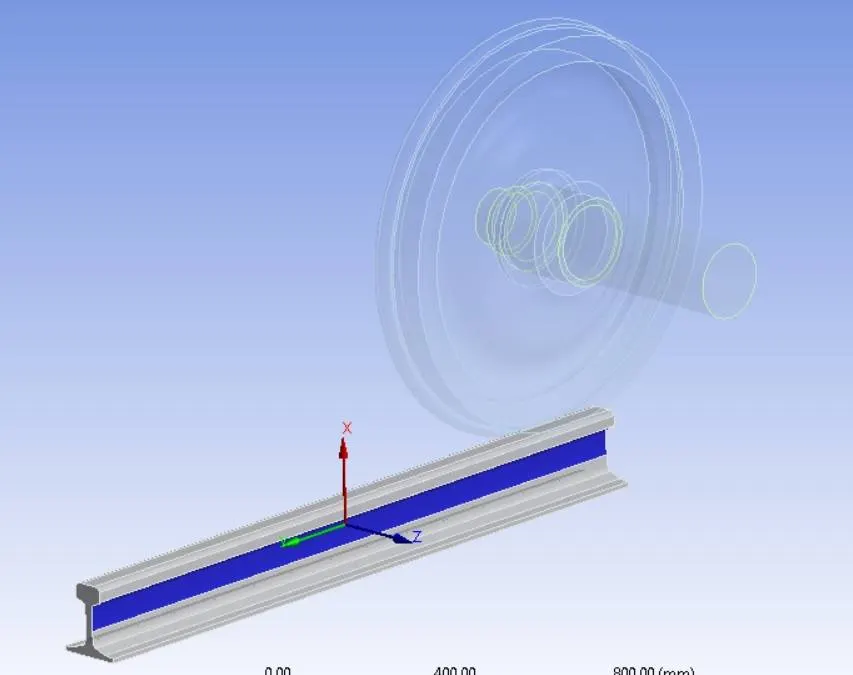
Fig 4. 1st Boundary Condition - Fixed Tracks
Translational Motion is given to Shaft in the negative X direction as shown in Figure 5
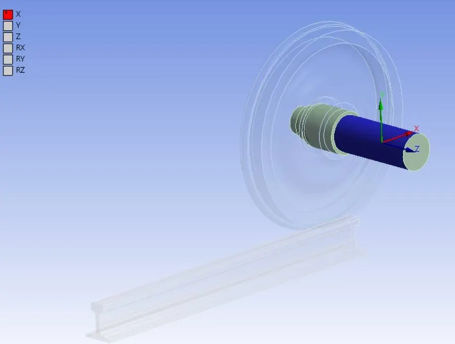
Fig 5. 2nd Boundary Condition - Shaft Translation
Planar motion is given to one of the faces of railwheel as shown in Figure 6
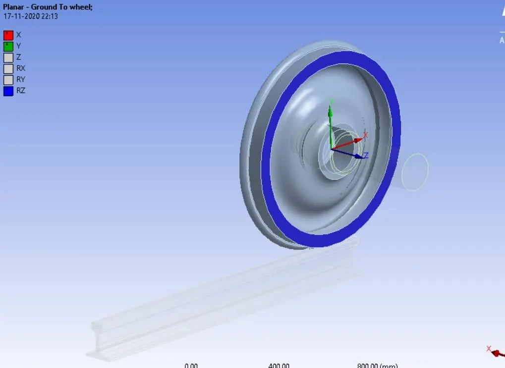
Fig 6. 3rd Boundary Condition - Planar
A joint displacement of 500 mm is given to the shaft in the negative X direction in subsequent steps of 100 mm so that the wheel can move along the track. Again bearing load of 100000 N is given to the bearing in negative y direction.
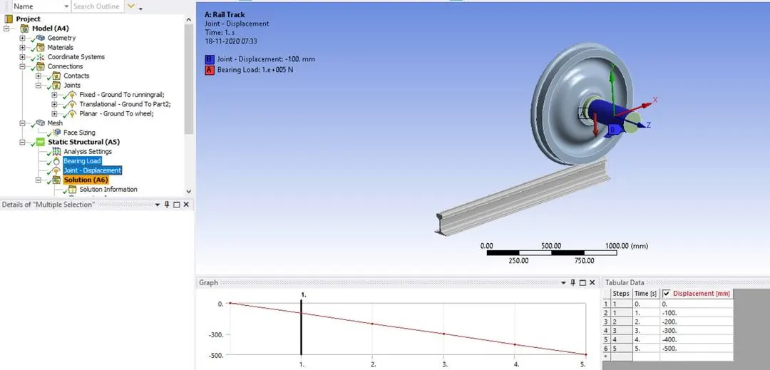
Fig 7. 4th Boundary Condition - Bearing Load and Joint Displacement
3. Analysis Settings
The settings used for performing the simulation is shown below.
| Definition | Settings |
| No of Steps | 5 |
| Auto Time Stepping | On (2nd to 5th step) |
| Define By | Time |
| Carry Over Time Step | On |
| Maximum Time Step | 1.00E-03 |
| Minimum Time Step | 0.1 |
| Large Deflection | On |
| Solver Type | Direct |
| Output Controls | Yes (All) |
4. Results of Case-1
In this case the bearing load applied is 100000 N and after appliying the boundary condition the model is solved to get total deformation, equivalent stress and life as shown in figure below.
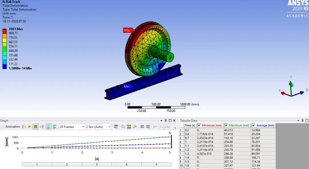
Fig 8. Total Deformation
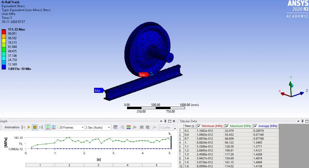
Fig 9. von-Mises Equivalent Stress
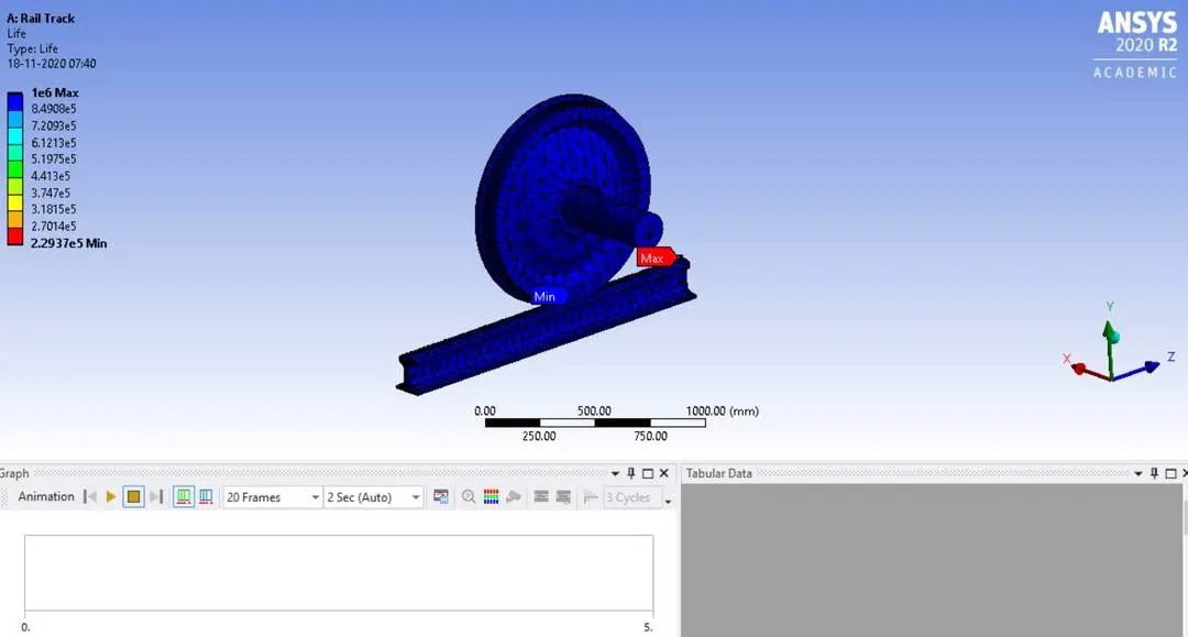
Fig 10. Life
5. Results of Case-2
In this case the bearing load applied is 500000 N and after appliying the boundary condition the model is solved to get total deformation, equivalent stress and life as shown in figure below.
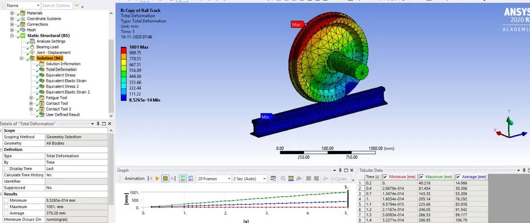
Fig 11. Total Deformation
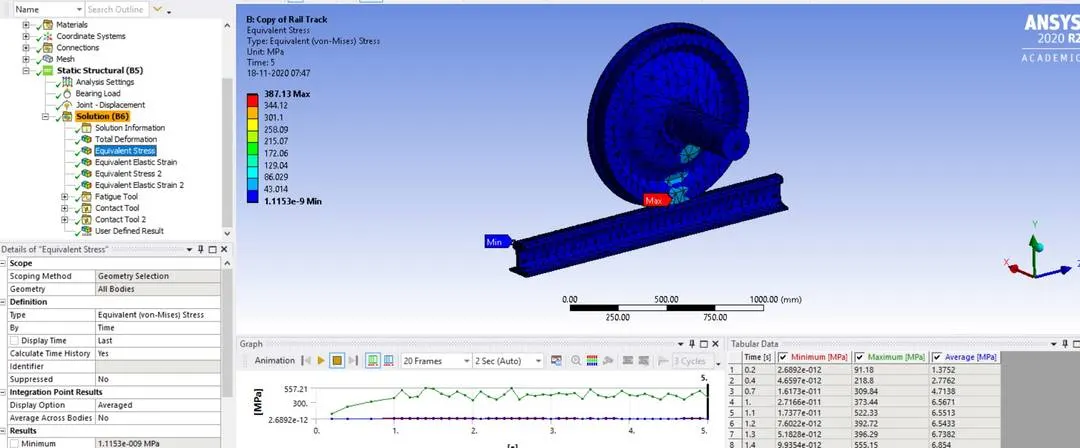
Fig 12. von-Mises Equivalent Stress
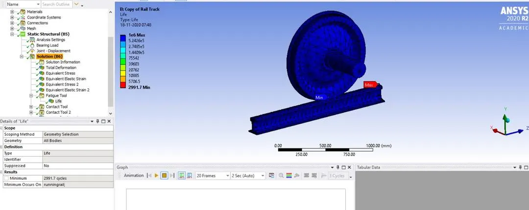
Fig 13. Life
6. UserDefined Results for Case 1
The total deformation is calculated for case 1 using the user defined formula and compared with the total deformation value given by ANSYS. The formula used for calculating the total displacement
is `sqrt(U X^2 + U Y^2 + UZ^2)`
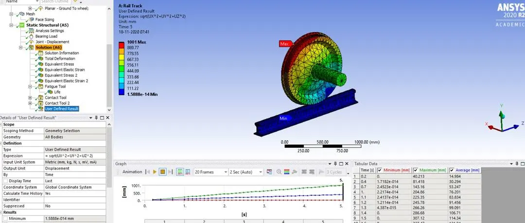
Fig 14. User Defined Results
It is observed that the value for total deformation of 1001 mm is same as that obtained from user defined result formula and ANSYS output.
7. Results and Discussions
The maximum total deformation and maximum life is same in both the cases but maximum von-Mises equivalent stress in Case 1 is 111.32 Mpa which is within the yield strength of Structural Steel (i.e, 250 MPa) but the stress in Case 2 exceeds the yield strength of the material. Thus it is advisable to use a bearing load of 100000 N.
| SL No | Parameters | Bearing Load | |
| 100000 N | 500000 N | ||
| 1 | Equivalent Stress (Mpa) | 111.32 | 387.13 |
| 2 | Total Deformation (mm) | 1001 | 1001 |
| 3 | Life (Cycles) | 1.00E+06 | 1.00E+06 |