Contact Stress in Rail-wheel and Track using Ansys

Objective

1. To mesh the model.
2. To apply the boundary conditions.
3. To do the analysis setting.
4. Evaluate the results.
5. To compare the total deformation, equivalent stress, and life of the wheel under 5E+05 N with 1E+05 N.
6. Implement the user-defined result and calculate the total deformation from this result and check if it is the same as that obtained by the in-built result by Ansys for a load of 1E+05 N.

Procedure

For solving this problem, the Static Structural module was chosen. In both the static structural modules, in Engineering Data, Structural Steel was the default material. It was kept as it is, as the material does not affect the stress concentration.

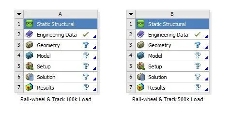
Figure 1: Static Structural module was chosen for this work.

The rail-wheel and track model was first imported and then opened in the Model section. Now, using the Model section of the Static Structural module, each part was first assigned the structural steel material. In the geometry, since the contact area was the area of interest, therefore, face sizing option was used in the contact region, with an element size of 35 mm. For the other region, the element size was kept equal to 50 mm.

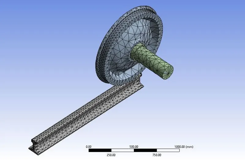
Figure 2: Rail-wheel and track model with a mesh size of 50 mm, and face sizing of 35 mm.

Boundary Conditions

Contact

In boundary conditions, firstly, the contact had to define. The Ansys automatically found out the neighboring faces of different bodies, that are in contact, and created a bonded contact between them. The automatic contact was perfect, only the type of contact had to change. So, for the wheel and track, bonded contact was changed to frictional contact with a coefficient of friction equal to 0.3. And for the contact between the wheel and the shaft, the bonded contact changed to frictionless.

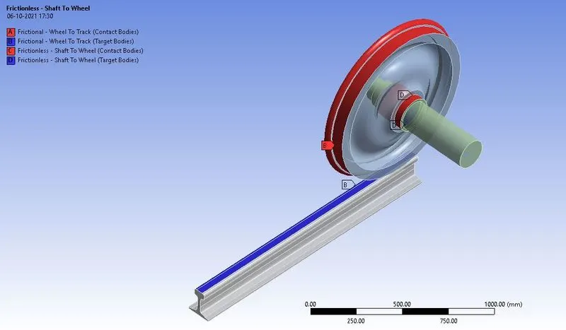
Figure 3: Wheel and track defined with frictional contact, and wheel and rail defined with frictionless contact.

Joint

While the railway moves, the track remains firm. Therefore, the track had to apply a fixed constraint. Using Connections → Body-Ground → Fixed, the track was fixed.

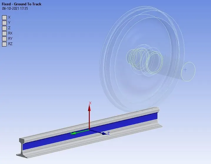
Figure 4: The track was constrained in all directions.

Next, the wheel should not de-rail, therefore, a Planar joint was applied to the wheel.

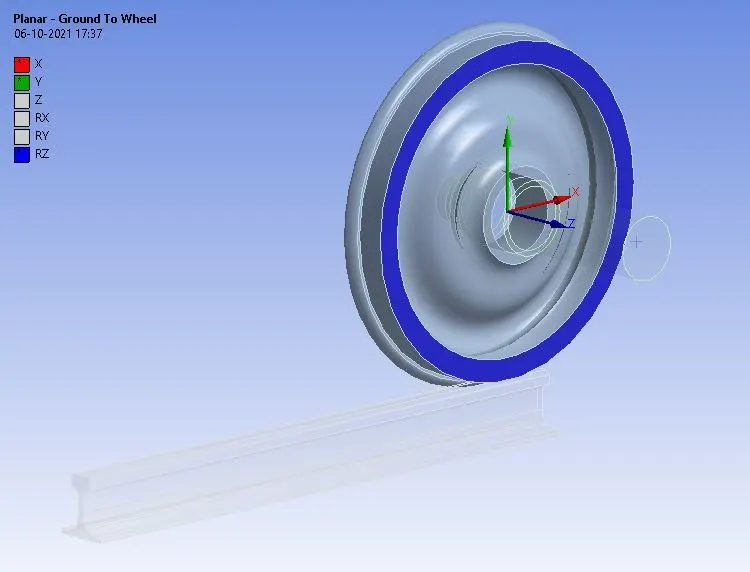
Figure 5: Planar joint to the wheel.

It is the shaft that was going to translate; therefore, the translation joint was applied to the shaft.

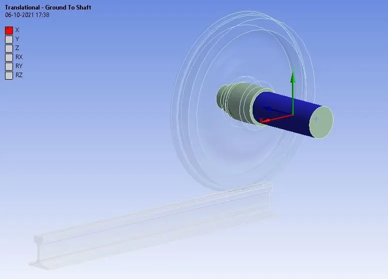
Figure 6: Translation joint to the shaft.

Now the problem was to solve in 5 steps, therefore in the analysis set, the Number of Steps was set to 5. Along with this, the minimum timestep was set to 1.0E-3 s, and the maximum time step was set to 0.1 s. And also, the large deflection was turned on.

Then the load has to define, therefore, using joint load displacement was given to the shaft in 5 steps as shown below.

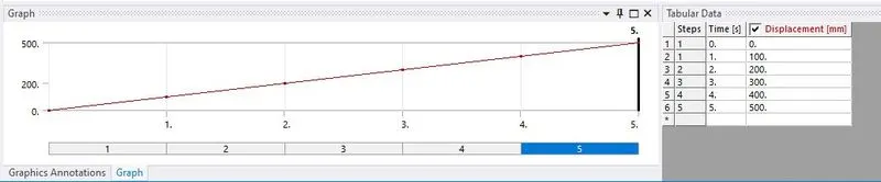
Figure 7: Displacement was given to shaft in 5 steps.

Another load that acts on this model is the bearing load. It is load that is carried by the bearing and then following to wheel. Therefore, a bearing load was applied onto the inner surface of the wheel, as shown below.

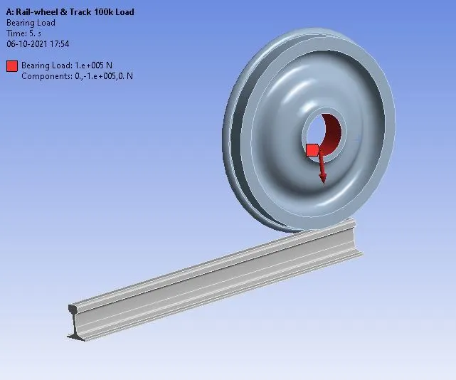
Figure 8: A bearing load of 1.00E+05 applied on the inner surface of the wheel.

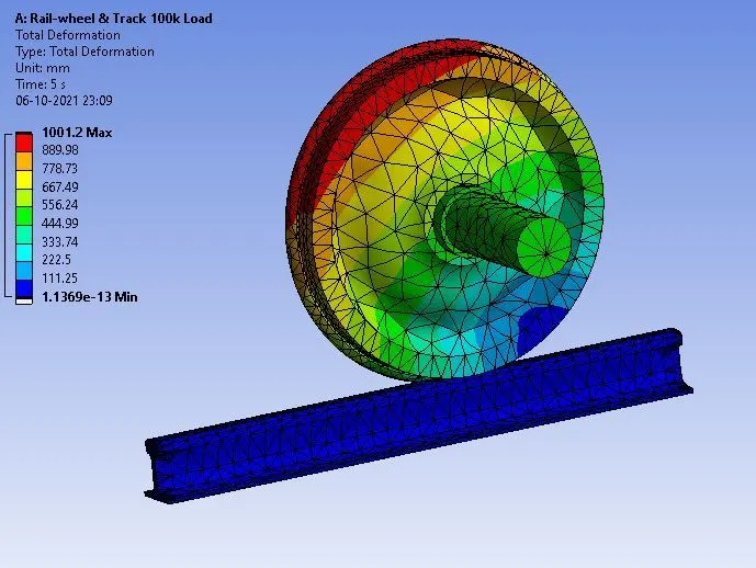
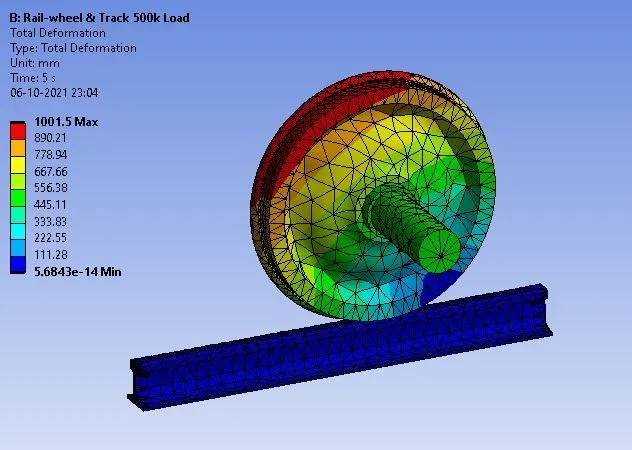
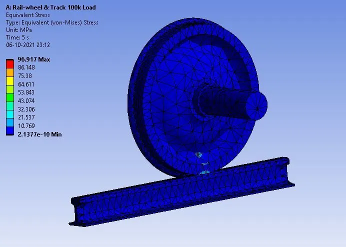
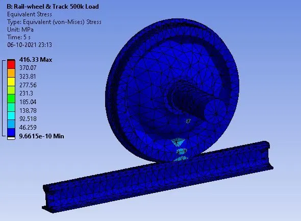
Once done with applying all the boundary conditions, the next thing was to request the output results. Under results, total deformation, equivalent stress, and the life of the wheel were requested. After setting all the required conditions, the problem was solved. The following figures show the total deformation, equivalent Von-Mises, and fatigue life contours of the model under two cases.

Figure 9: Total deformation contour of the model under 1.0E+05, and 5.0E+05 bearing load, respectively.

Figure 10: Equivalent Von-Mises stress contour of the model under 1.0E+05, and 5.0E+05 bearing load, respectively.

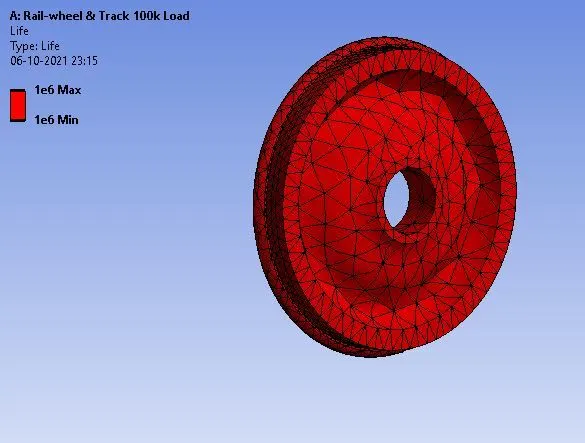
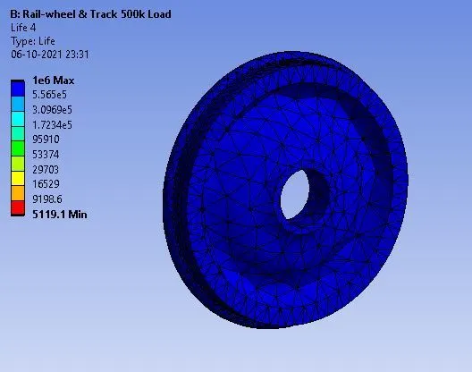
Figure 11: Life of the wheel under 1.0E+05, and 5.0E+05 bearing load, respectively.

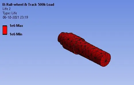
Figure 12: Life of the shaft under 1.0E+05, and 5.0E+05 bearing load, respectively.

The figures above clearly show the effect of increasing the bearing load on the stresses developed and the life of each part. The maximum stress developed in the case of 1.0E+05 N bearing load was 96.917 ≈ 97 MPa. When the load was increased 5 times the earlier case, the stress increased to 416.33 MPa, which is approx. time the previous stress.

The increased induced stress means a decreased life. When the bearing load was 1.0E+05, the minimum life of the wheel was 1.0E+06 cycles, but when the bearing load was increased to 5 times, the minimum life of the wheel was reduced to 5119 cycles. There was no significant change in the life of the shaft. The figures above clearly show the effect of increasing the bearing load on the stresses developed and the life of each part. The maximum stress developed in the case of 1.0E+05 N bearing load was 96.917 ≈ 97 MPa. When the load was increased 5 times the earlier case, the stress increased to 416.33 MPa, which is approx. time the previous stress.

The last objective of this work was to implement the user-defined result and calculate the total deformation from this result and check if it is the same as that obtained by the in-built result by Ansys for a load of 1E+05 N.

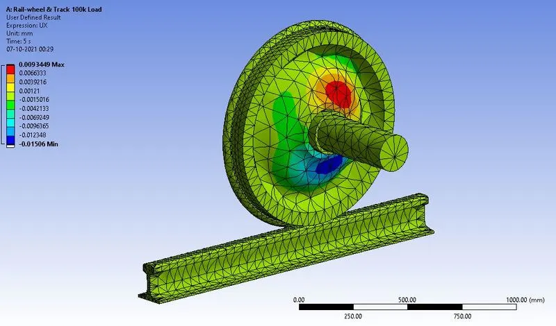
Figure 13: User-defined result.