Simulating application of Karman's vortex : Flow over a Cylinder
Aim
To simulate flow over a cylinder and explain Karman’s vortex street.
To understand vortex shedding for different Reynolds number by changing the inlet velocities accordingly.
To create a monitor point behind the cylinder at a distance of 4 times the diameter of cylinder from which we can calculate and analyze vortex shedding.
Objective –
- Simulate the flow with the steady and unsteady case and calculate the Strouhal Number for Re= 100.
- Calculate the coefficient of drag and lift over a cylinder by setting the Reynolds number to 10,100,1000,10000 & 100000. (Run with steady solver)
- Discuss the effect of Reynolds number on the coefficient of drag. [ Results should be validated with any standard literature and error should be within 5 %]
- In both approaches, show that the flow has converged. That is, what quantities or plots need to be looked at to determine that the flow has converged?
- Plots of the coefficient of drag and lift.
- Plots to show vortex shedding behind the cylinder.
- Mention the referred material at the end of the challenge submission page.
Theory
In fluid dynamics, a Von Karman’s Vortex Street is a repeating pattern of swirling vortices shedding caused by vortex shedding which is responsible for unsteady separation of flow of fluid around bluff bodies. This phenomenon is named after engineer and fluid dynamists Von Karman
What Exactly is a Karman Street?
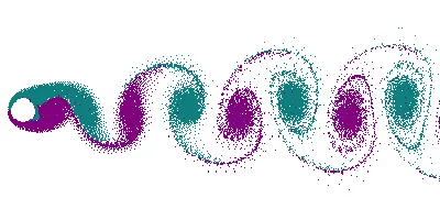
Consider a stream of fluid flow past a circular cylinder, which can be called the archetypal or quintessential bluff body - a cross-section of 'perfect platonic circle' as R Narasimha aptly puts it in his two-part article. In the wake of the cylinder, the flow pattern consists of an alternating system of vortices or regions of rotation, as shown in Figure.
A clockwise rotating eddy or vortex is 'shed' from the top side, followed by an anticlockwise rotating vortex from the bottom side, and this process continues leading to a staggered system of alternating vortices.
It is important to note that even if the oncoming flow is steady (i.e., does not change with time), the unsteadiness is intrinsically generated and the Karman Street is formed downstream of the body.
Physics behind Vortex Formation?
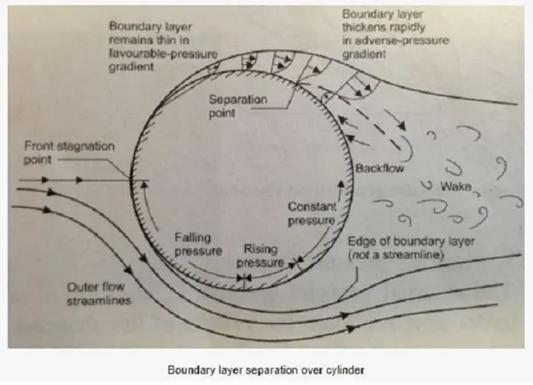
In the shown in the figure. we can see that as a fluid particle flow towards the leading edge of the cylinder, the pressure in the particle rises from the free stream pressure to stagnation pressure. The high fluid pressure near the leading edge impels that flow about the cylinder as boundary layers develop on both sides. The high pressure is not sufficient to force the flow about back of cylinder at high Reynolds numbers.
Near the widest section of the cylinder, the boundary layers separate from each side of the cylinder surface and form two shear layer that trail aft in the flow and bound the wake. Since the inner most portion of shear layer in contact with cylinder, which moves much slower than that of the outer most portion of shear layer in contact with free flow. The shear rolls into near wake, where the fold on to each other and coalesce into discrete swirling vortices. A regular pattern of vortices called the vortex street trails aft in the wake.
Strouhal Number -
Is a dimensionless value useful for analysing oscillating unsteady fluid flow dynamics problems?
The Strouhal Number represents a measure of the ratio of the inertial forces due to the unsteadiness of the flow or local acceleration to the inertial forces due to changes in velocity from one point to another in the flow field.
The Strouhal Number can be expressed as
St = ω l / v (1)
Here
St = Strouhal Number
ω = oscillation frequency
l = characteristic length
v = flow velocity
- For large Strouhal numbers (order of 1), viscosity dominates fluid flow resulting in collective oscillating movement of the fluid.
- For low Strouhal numbers (order of 10^-4 and below), the high speed quasi-steady-state portion of the movement dominates the oscillation.
- Oscillations at intermediate Strouhal numbers is characterized by buildup and rapidly subsequent shedding of vortices.
Coefficient of Drag -
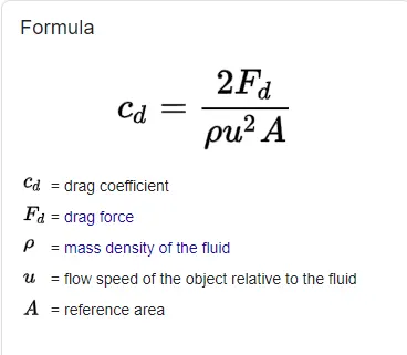
In fluid dynamics, the drag coefficient (commonly denoted as: [`C_d` or `C_x` or `C_w`] is a dimensionless quantity that is used to quantify the drag or resistance of an object in a fluid environment, such as air or water. It is used in the drag equation in which a lower drag coefficient indicates the object will have less aerodynamic or hydrodynamic drag. The drag coefficient is always associated with a particular surface area
The drag coefficient of any object comprises the effects of the two basic contributors to fluid dynamic drag: skin friction and form drag. The drag coefficient of a lifting airfoiled or hydrofoil also includes the effects of lift-induced drag. The drag coefficient of a complete structure such as an aircraft also includes the effects of interference drag
Coefficient of Lift –
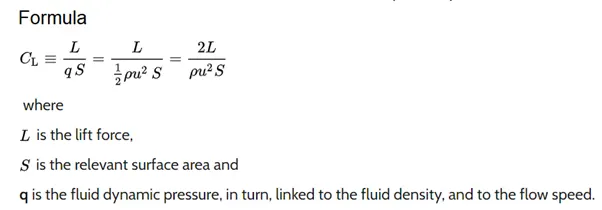
The lift coefficient (`C_L`) is a dimensionless coefficient that relates the lift generated by a lifting body to the fluid density around the body, the fluid velocity and an associated reference area. A lifting body is a foil or a complete foil-bearing body such as a fixed-wing aircraft. CL is a function of the angle of the body to the flow, its Reynolds number and its Mach number. The section lift coefficient cl refers to the dynamic lift characteristics of a two-dimensional foil section, with the reference area replaced by the foil chord.
Procedure –
Problem Setup –
(1) Geometry
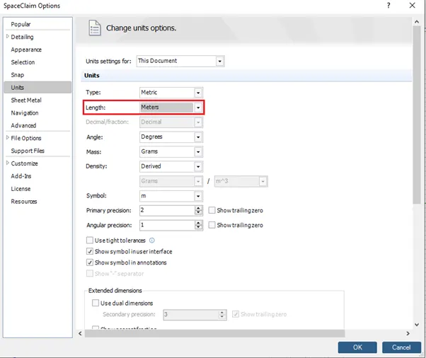
- Files → Space Claim Options → Units
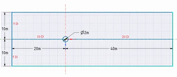
Create a geometry in Space Claim with following dimensions,
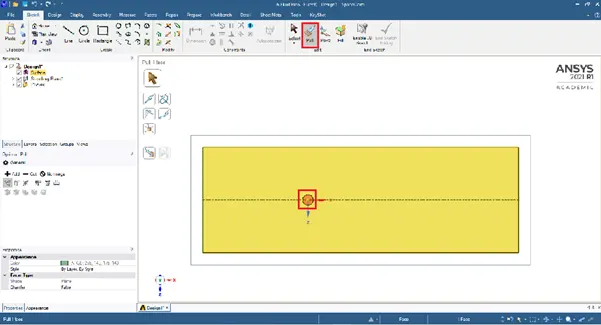
Use Pull tool to extract the surface of cylinder, and delete all the construction lines used to create the boundary around the circular cylinder. With this geometry creation is done, close Space Claim.
(2) Mesh Generation –
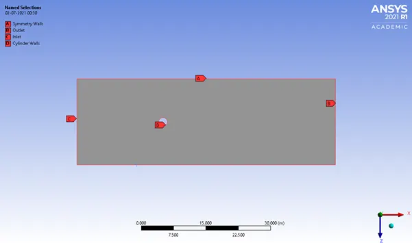
- Right Click → Insert → Named Selection, As follows
Recommended, generate mesh with default settings and check the simulation for only first case. If not sure how mesh element sizing and other mesh techniques are used to enhance the quality of mesh.
(3) Mesh Setting –
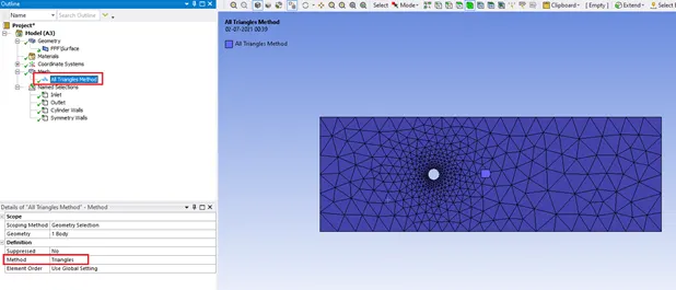
Methods -
- Right Click → Insert → Methods,
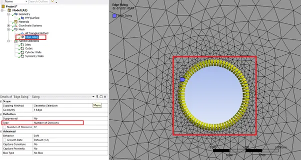
Sizing -
- Right Click → Insert → Sizing,
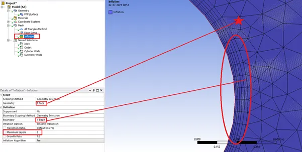
Inflation -
- Right Click → Insert → Inflation
Before –
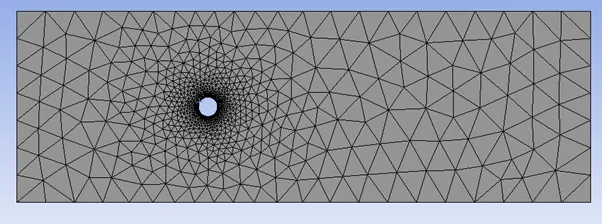
After –
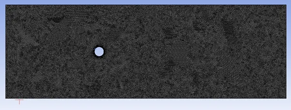
Using an Element Size – 0.2 m (Constant) throughout all simulation cases.
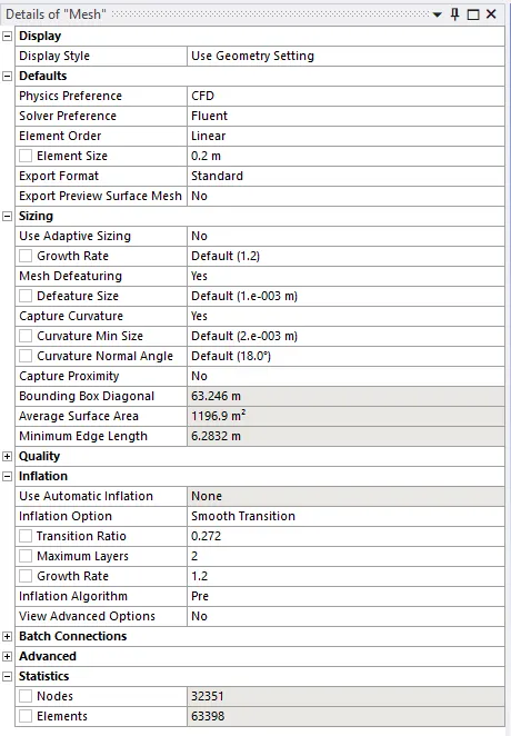
(4) Mesh Details -
(5) Solution Setup -
(1) General → Solver → Pressure-based → Time→ Steady State
(2) Models → Viscous → Laminar
(3) Material → Fluid → Add New → Fluent Database → User-Material (In our case user-material has Density=1 kg/m^3 & Viscosity=0.02 Kg/m-s)
(4) Cell Zone Conditions → fff_surface → Fluid → User-material
(5) Boundary Conditions
a). Intel (Velocity= User-defined)
b). Outlet (Gauss Pressure=1 atm)
c). Cylinder_walls → Wall Motion → Stationary → Shear Condition → No Slip
d). Symmetry_Walls → Symmetry boundary
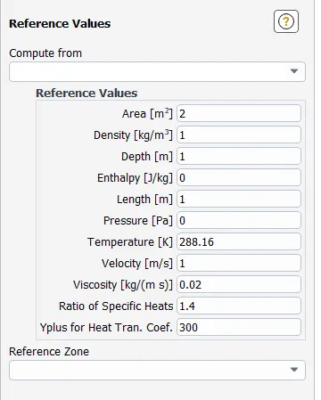
(6) Reference Values →
(7) Method → Scheme → Simple
(8) Results → Create → Point → X(m)= 4 times cylinder diameter → Y(m)= 0
(9) Solution → Definition →
a). Surface Report → Vertex Average → Velocity/Velocity magnitude → Field Variable = monitor-point
b). Force Report → Lift → Lift Coefficient → Field Variable = Cylinder_Walls
c). Force Report → Drag → Drag Coefficient → Field Variable = Cylinder_Walls
(10) Initialize Solution → Hybrid
(11) Results →
a). Create Contour → Velocity → Field Variable = All Named Selections
b). Create Contour → Pressure → Field Variable = All Named Selections
c). Activities → Create Animation → Solution Animation → Velocity Contour
-------------------------------------------------X-------------------------X-----------------------------------------------------------------
Part 1- Simulate flow over cylinder with Steady and Unsteady State with a Reynold’s Number of 100 respectively and also calculate Strouhal Number for same.
- Steady State
Reynold’s Number-100
Velocity = 1 m/s
No of Time Step =1500
Time Step = 1 second
Hybrid Initialization
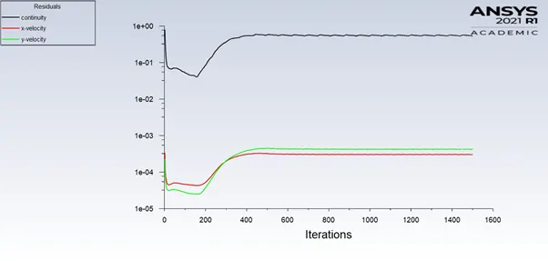
Residual Plot
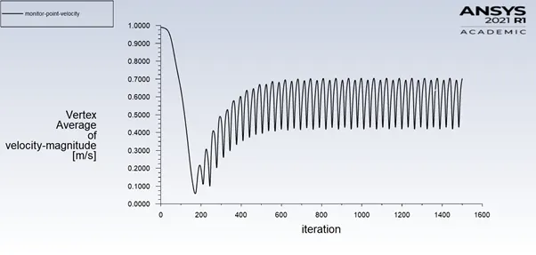
Monitor Point Velocity Plot
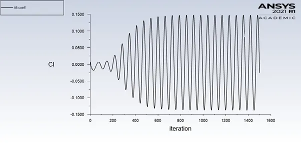
Lift Coefficient Plot
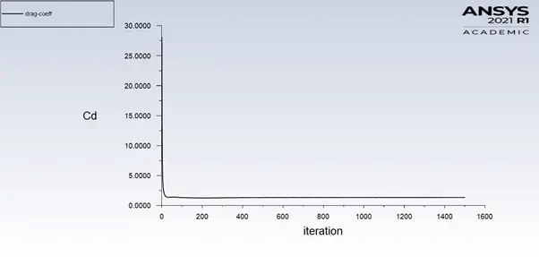
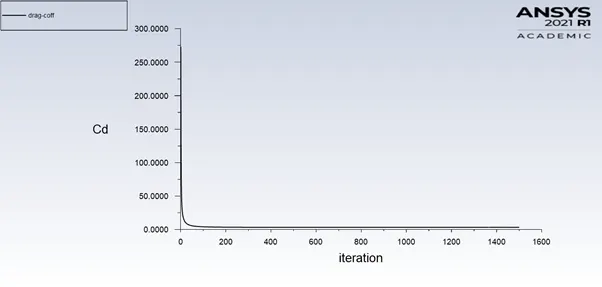
Drag Coefficient Plot
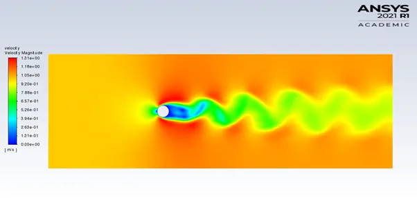
Velocity Contour
Pressure Plot
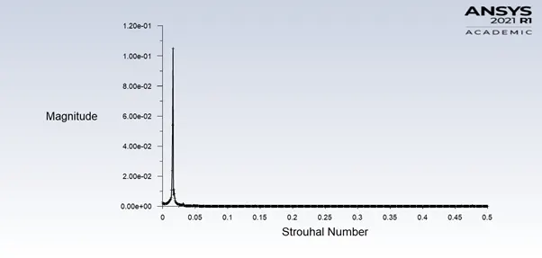
FFT Plot for Coefficient of Lift (Time-Data)
Inference from above Steady State study: -
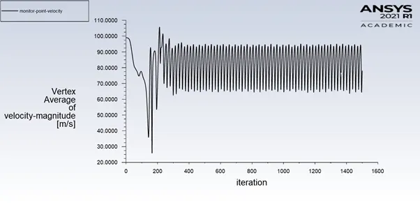
- In monitor-velocity plot at a particular point from the walls of cylinder, we can see that the velocity magnitude keeps on fluctuating with the flow causing phenomenon called Vortex Shedding.
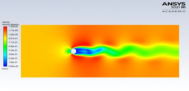
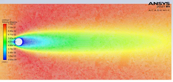
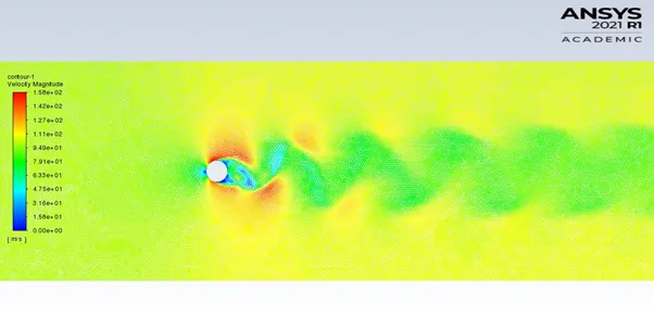
- Velocity contour, shows a clear picture of Vortex shedding taking place and the region of vortices increase with the distance travelled by flow vortex. Vortex Shedding is denoted by a green color map.
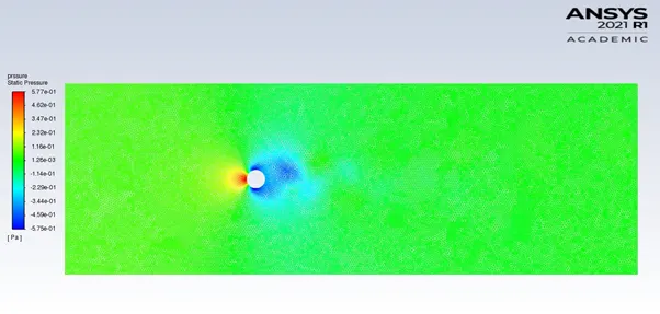
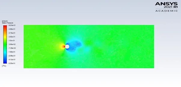
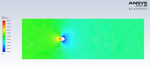
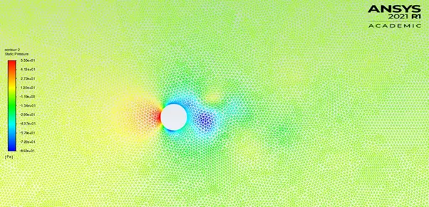
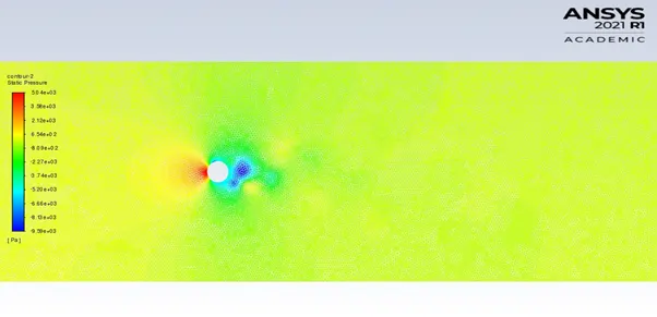
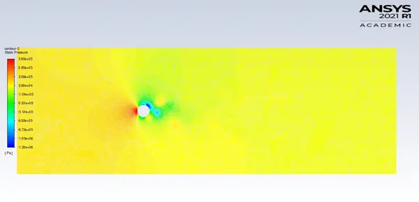
- In Pressure contour, we can notice due to flow impact on cylinder and around its wall, there is higher pressure region created and in turn results in a pressure dropped region behind and around the cylinder.
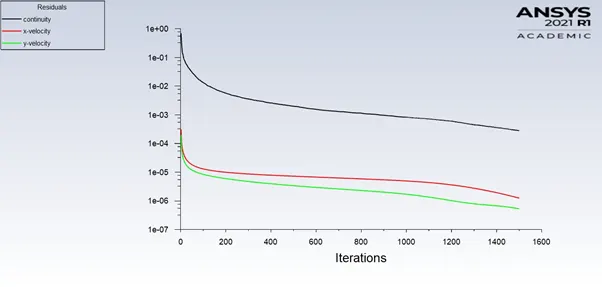
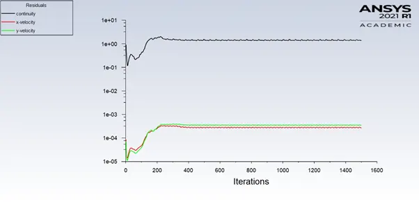
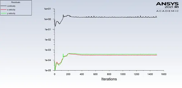
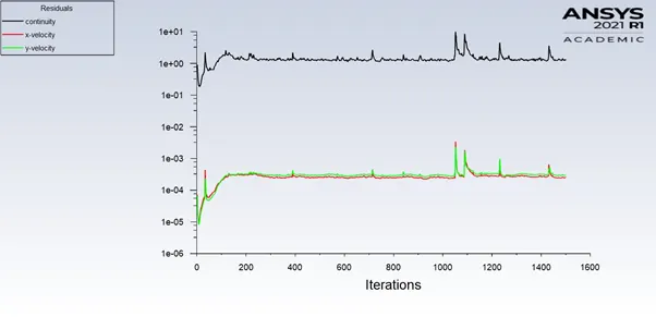
- When we look at convergence in steady state simulation, the residuals steadily fluctuating but most them don’t fall under 1E-4. Hence, one has to check the quantity of interest and else change parameters accordingly.
- Coefficient of Drag = 1.342987
- Coefficient of Lift = -0.025176
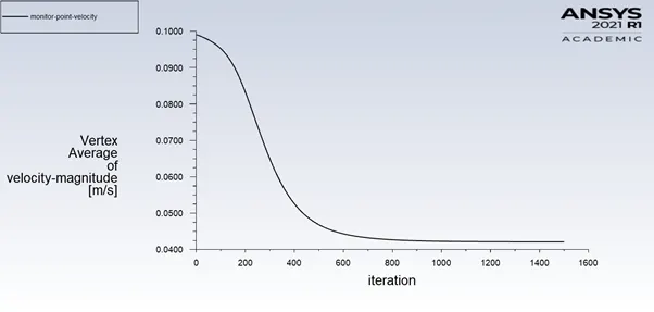
- Vertex Average Velocity Magnitude = 0.7028
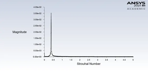
- Strouhal Number = 0.0160 (Maximum Magnitude 1.34E-01)
2. Transient State
Reynold’s Number-100
Velocity = 1 m/s
No of Time Step =1000
Time Step = 0.5 second
Hybrid Initialization
Residual Plot
Monitor Point Velocity Plot
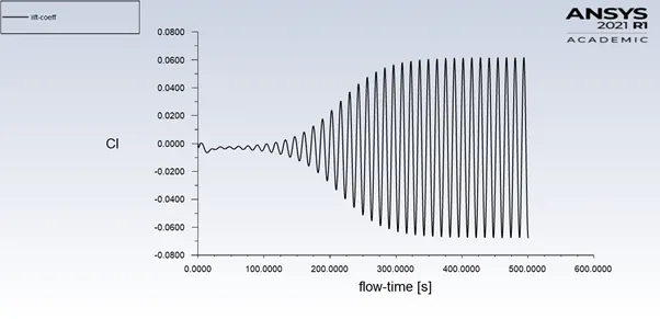
Lift Coefficient Plot
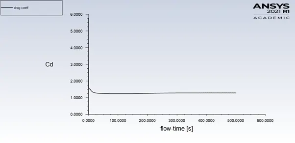
Drag Coefficient Plot
Velocity Contour
Pressure Plot
FFT Plot for Coefficient of Lift (Time-Data)
Inference from above Transient State study: -
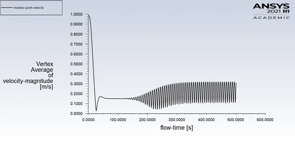
- In monitor-velocity plot at a particular point from the walls of cylinder, we can see that the velocity magnitude keeps on fluctuating with the flow causing phenomenon called Vortex Shedding.
- Transient state simulation is a time constraint simulation. Why so? We can observer right after initialization, that each result point data is recorded/updated with each time step. Also makes this simulation more accurate and computational hectic.
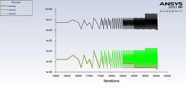
- When we look at convergence in transient simulation, the residuals steadily fluctuate in the range 1E-05. hence, the simulation has well converged.
- Coefficient of Drag = 1.2875384
- Coefficient of Lift = -0.067790
- Vertex Average Velocity Magnitude = 0.309839
- Strouhal Number = 0.3784607 (Maximum Magnitude 3.51E-02)
-------------------------------------------------X-------------------------X-----------------------------------------------------------------
Part 2 – Calculate the coefficient of drag and lift over a cylinder by setting the Reynold’s number to 10,100,1000,10000,100000 and run the simulation with Steady State Solver.
1. Reynold’s Number =10
Residual Plot
Monitor Point Velocity Plot
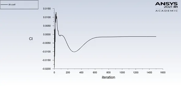
Coefficient of Lift Plot
Coefficient of Drag Plot
Velocity Contour
Pressure Contour
-------------------------------------------------X-------------------------X-----------------------------------------------------------------
2. Reynold’s Number =100
Residual Plot
Monitor Point Velocity Plot
Coefficient of Lift Plot
Coefficient of Drag Plot
Velocity Contour
Pressure Contour
-------------------------------------------------X-------------------------X-----------------------------------------------------------------
3. Reynold’s Number =1000
Residual Plot
Monitor Point Velocity Plot
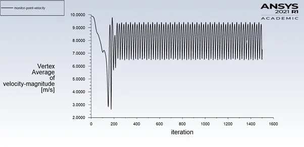
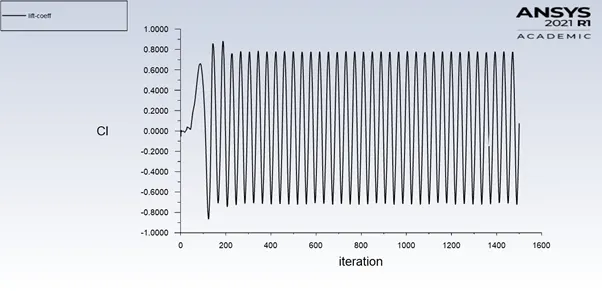
Coefficient of Lift Plot
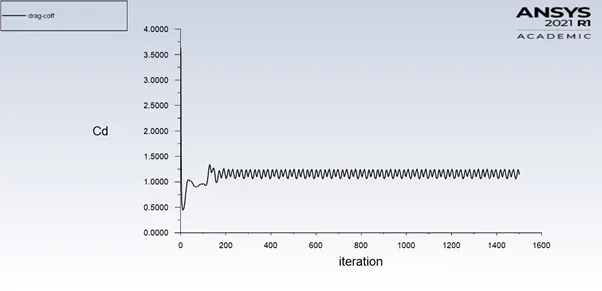
Coefficient of Drag Plot
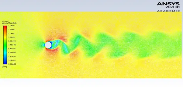
Velocity Contour
Pressure Contour
-------------------------------------------------X-------------------------X-----------------------------------------------------------------
4. Reynold’s Number =10000
Residual Plot
Monitor Point Velocity Plot
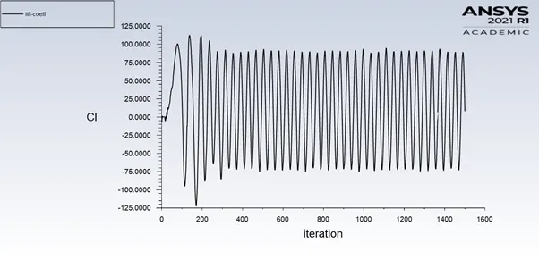
Coefficient of Lift Plot
Coefficient of Drag Plot
Velocity Contour
Pressure Contour
-------------------------------------------------X-------------------------X-----------------------------------------------------------------
5. Reynold’s Number =100000
Residual Plot
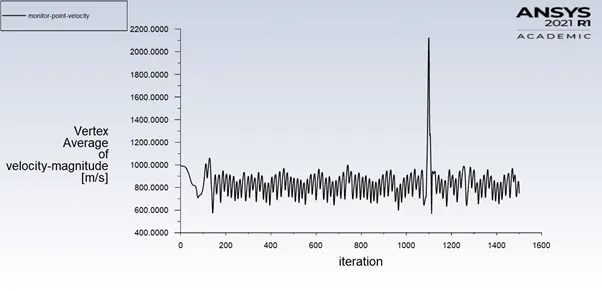
Monitor Point Velocity Plot
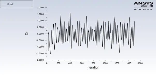
Coefficient of Lift Plot
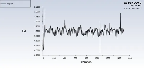
Coefficient of Drag Plot
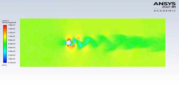
Velocity Contour
Pressure Contour
Conclusion –
Discuss the effect of Reynolds number on the coefficient of drag. [ Results should be validated with any standard literature and error should be within 5 %]
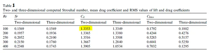
Literature Table for reference
Simulation Results
Part 2 -
|
Reynold’s Number |
Coefficient of Drag |
Coefficient of Lift |
Vertex Average Velocity (V)-m/s |
|
10 |
3.3332705 |
-0.001255 |
0.04212616 |
|
100 (A) |
1.343987 |
-0.025176 |
0.70287621 |
|
100 (B) |
1.2875384 |
-0.067790 |
0.30983990 |
|
1000 |
1.1430739 |
0.0753713 |
7.3803769 |
|
10000 |
1.0166918 |
0.0786433 |
78.125677 |
|
100000 |
1.0999667 |
0.0942583 |
747.87158 |
In the below table error margin accepted is of ± 5%
Part 1 -
|
Reynold’s Number |
Analytical |
Run |
Error Margin (%) |
Strouhal Number |
|
100 (A) |
1.3353 |
1.343987 |
+ 0.6505 |
0.0160997 |
|
100 (B) |
1.3353 |
1.2875384 |
- 3.5768 |
0.3784607 |
Here 100 (A) – Flow over Cylinder with Steady State Simulation
100 (B) – Flow over Cylinder with Transient State Simulation
Inference -
- Importance of Convergence and How to detect the same?
- When your simulation has no changes on all convergence criteria, after certain iteration or time step, which results the simulation to reach steady-state i.e., in other words simulation is converged.
- Following are the RMS residual levels one can consider to predict convergence
- (1) 1E-04 – Loosely Converged
- (2) 1E-05 – Well Converged
- (3) 1E-06 – Tightly Converged
- In our case for Re=100 Steady State simulation, residuals are steady but do not fall under 1E-04. Thus, we check other point of interest rather than residuals i.e.
- (1) Coefficient Of Drag
- (2) Coefficient of Lift
- (3) Vertex Average of Velocity
- All three plot parameters do not show any abnormal variation throughout run iterations. Hence, we can say that simulation is converged
- Similarly in case Re=100 Unsteady State simulation, residuals are fluctuating but are in well range of 1E-05. Which is consider to be well converged
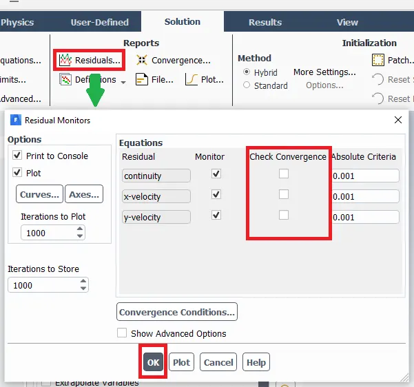
- Once we know that initial simulation is getting converged, for further simulation and case variations, we can unmark convergence check criteria from Solution → Residuals
- We also get know that with precise refinement of mesh, the computational time and iteration increases for the same.
- The behaviour of simulation results with Reynold’s Number increasing are as follows –
- (1) Pressure of impact on the walls decreases vies-versa the flow separation increases.
- (2) Higher fluctuation in Vortex Shedding but the vortices size decreases.
- (3) Coefficient of drag decreases
- (4) Coefficient of lift increases
- Whereas, when the Reynold’s Number is 10, Vortex Shedding is not achieved and can be achieved by having the higher flow velocity at the inlet.
- Comparing the Steady and Transient State simulation for Reynold’s Number = 100: -
- (1) As the flow gets stable, Steady State results for its activities are recorded and moreover this simulation has no time constraint.
- (2) In Transient State, results of Plots and Contours are captured from “Time Step = 0 sec”.
- Vortex Shedding and Street Formation: -
- (1) For Reynold’s Number = 10 no Vortex Shedding is seen and only street formation is seen
- (2) Whereas as the Reynold’s Number increases so thus the Vortex Shedding.
- (3) In the case of Reynold’s Number =10000, Vortex Shedding fluctuation have dropped frames and Street formation is not prominently seen.
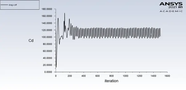
- (4) In Reynold’s Number = 100000 case, we observe the plot frames to have short heighted peaks rather tall ones seen in previous cases.
References -
- Numerical simulation of laminar flow past a circular cylinder [https://www.sciencedirect.com/science/article/pii/S0307904X08000243]
- Numerical Simulation of Flows past a Circular and a Square Cylinder at High Reynolds Number, and a Curved Plate in Transitional Flow. [https://core.ac.uk/download/pdf/233210828.pdf]
- High Reynolds number turbulent flow past a rotating cylinder [https://www.sciencedirect.com/science/article/pii/S0307904X11004124]
- H.K. Williamson - Vortex dynamics in the cylinder wakes - [https://www.annualreviews.org/doi/pdf/10.1146/annurev.fl.28.010196.002401]
- Vortex Shedding - [https://www.thermopedia.com/content/1247/]
- A Stroll down Karman Street - Raghuraman, N Govardhan and 0 N Ramesh - [https://www.ias.ac.in/article/fulltext/reso/010/08/0025-0037]