Week 2 - Flow over a Cylinder.

Flow Over a Cylinder: Simulation Report

1. Aim

The aim of this study is to simulate and analyze the flow over a circular cylinder for various Reynolds numbers, focusing on the Kármán vortex street phenomenon and its related parameters, such as the Strouhal number, drag, and lift coefficients.

2. Introduction & Theory

Flow over a circular cylinder is an important topic in fluid mechanics due to its practical applications, including aerodynamics, structural analysis, and environmental engineering. At specific Reynolds numbers, the flow forms alternating vortices known as the Kármán vortex street, a recurring phenomenon for bluff body flows.

• Kármán vortex street occurs in the wake of the cylinder as alternating low-pressure zones form, resulting in oscillating lift forces. Understanding this vortex shedding pattern is critical for many practical applications like bridge construction, aircraft design, and marine structures.

• The Reynolds number (Re) governs the flow regime and is defined as:
  `Re = (rho * U * D)/mu` Where:

• `rho` = density of the fluid,

• `U` = free-stream velocity,

• `D` = diameter of the cylinder,

• `mu` = dynamic viscosity of the fluid.

• The Strouhal number (St), which describes the frequency of vortex shedding, is computed as:
  `St = (f * D)/U`
  Where:

• `f` = vortex shedding frequency,

• `D` = cylinder diameter,

• `U` = free-stream velocity.

The drag coefficient (C_d) and lift coefficient (C_l) are key parameters in understanding the aerodynamic forces acting on the cylinder:

`C_d = (F_d)/(0.5 * rho * U^2 * A)`

`C_l = (F_l)/(0.5 * rho * U^2 * A)`

Where:

• `F_d` = drag force,

• `F_l` = lift force,

• `A` = reference area (for a cylinder, it's based on diameter)

• 
  

3. Simulation Setup for Flow Over a Cylinder

Software Used: ANSYS Fluent is used for 2D simulations of flow over a circular cylinder.

Geometry: The cylinder has a radius of 1 meter, and the computational domain is 20 meters wide by 40 meters long, large enough to avoid boundary interference with the flow.

Mesh/Grid Details: A structured mesh with 17,690 nodes and 17,568 elements is used. The grid is refined near the cylinder to capture boundary layer effects and wake vortices accurately. A mesh independence study confirmed solution accuracy.

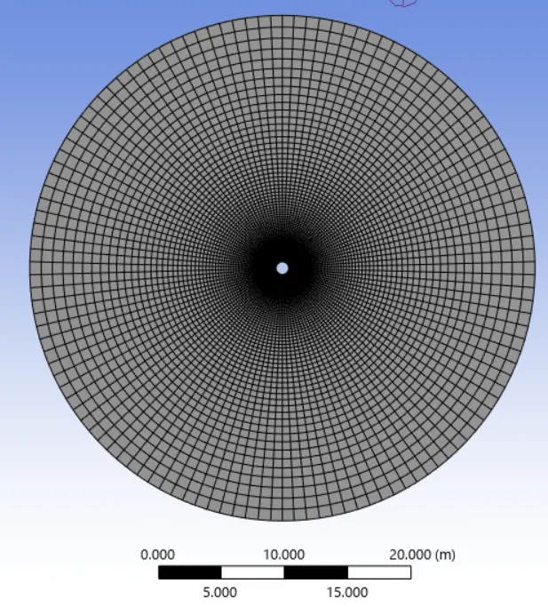
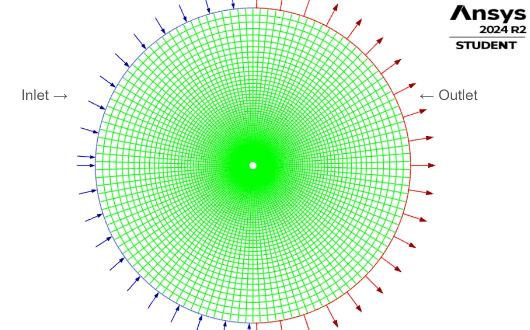
Figure1: showing image of mesh.

Solver Settings

• Flow Type: Incompressible.

• Solvers:

• Steady-state for low Reynolds numbers (Re) with laminar flow.

• Unsteady solver for higher Re where vortex shedding occurs.

• Pressure-Velocity Coupling: SIMPLE scheme.

• Unsteady Time Step: Delta t = 0.001 seconds.

Reynolds Number Variation

Reynolds number is controlled by varying inlet velocity, with the cylinder diameter and fluid properties kept constant. Simulations are run for Re = 10 to 100,000, covering laminar to turbulent flows.

Boundary Conditions

• Inlet: Uniform velocity (varied based on Re).

• Outlet: Pressure outlet at atmospheric pressure.

• Side Walls: Symmetry boundary to prevent interference with flow.

• Cylinder Surface: No-slip boundary condition to capture boundary layer and separation effects.

4. Results

The simulation was done for one unsteady case and five unsteady cases.

Here I am giving the plots of Residual, X velocity, Cd, and CL of only unsteady at Re 100 and Steady at Re 100 for comparison

Residuals are given to prove the convergence. And the contour plot of X velocity is given for a qualitative analysis..

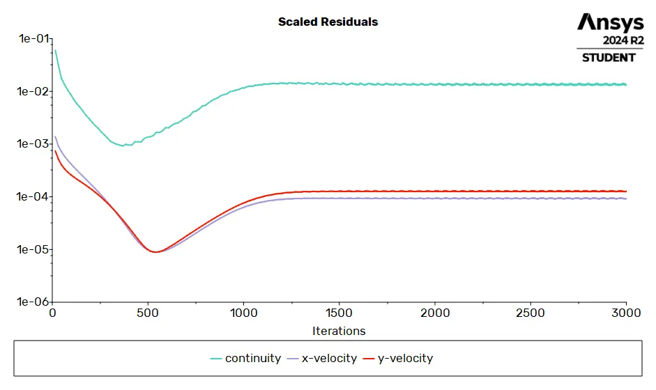
Figure 1: showing image x velocity of Steady state at Reynolds number 100.

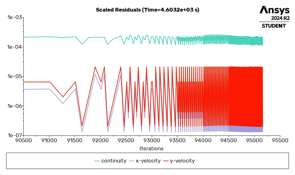
Figure 2: showing image x velocity of Unsteady state at Reynolds number 100.

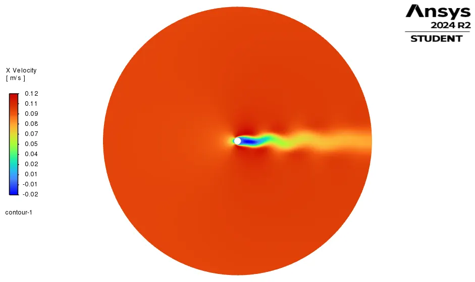
Figure 3: showing image x velocity of Steady state at Reynolds number 100.

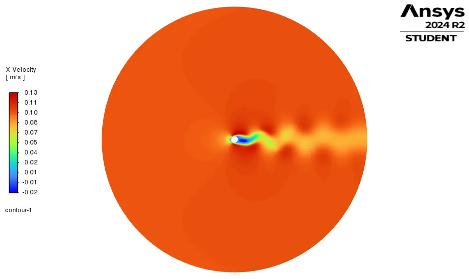
Figure 4: showing image x velocity of Unsteady state at Reynolds number 100.

Here we can see that vorticity is captured better in transient flow.

Part 1 of Challenge

Simulate the flow with the steady and unsteady case and calculate the Strouhal Number for Re= 100.

The Strouhal number was calculated to be 0.016 for Re equal to 100. {Strouhal number can also be calculated from FFT frequency, here I am calculating it manually}

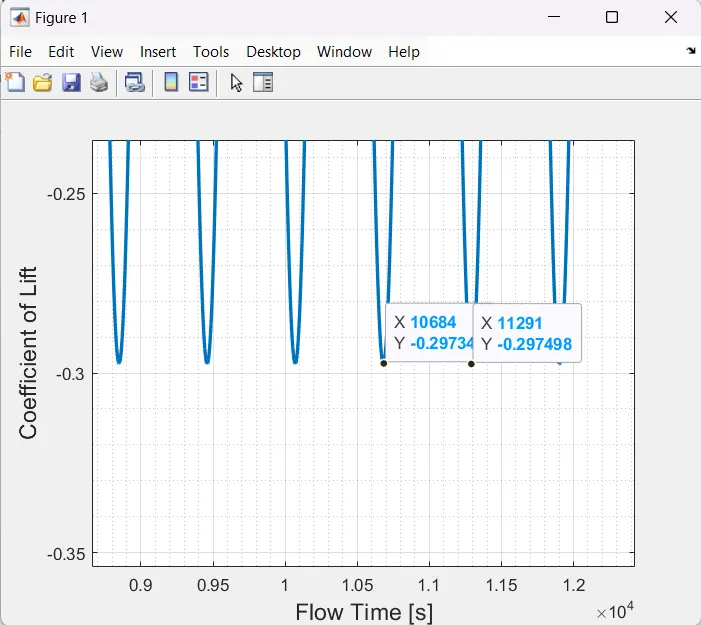
Time for 1 oscillation x2-x1= 11291-10684=607; therefore frequency is 1/607=0.001647

Sr = Strouhal Number=0.001647*1*10^1= 0.01647

Since there is no frequency over time of flow in steady state.

Part 2 of Challenge

1. Calculate the coefficient of drag and lift over a cylinder by setting the Reynolds number to 10,100,1000,10000 & 100000. (Run with steady solver)

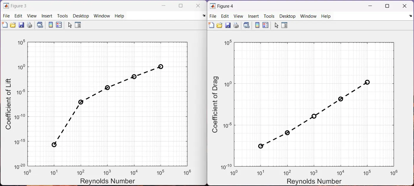
Figure 5: showing the change of cd and cl with respect to Reynold’s number.

2. Discuss the effect of Reynolds number on the coefficient of drag. [ Results should be validated with any standard literature and error should be within 5 %]

As Reynolds number increases, coefficient of drag increases, which is the same trend as in the standard literature suggested in the question.

The suggested literature was using URANS (Unsteady RANS) and in the challenge I have done URANS only for one case that is RE 100, for which I got the result within the 5% error limit.

In all other cases in which I have used steady RANS, I have larger errors.

5. Conclusion

The study aimed to investigate the flow behavior around a cylinder at different Reynolds numbers (Re) and calculate key parameters such as the Strouhal number, drag coefficient (CD), and lift coefficient (CL). The results can be summarized as follows:

Part 1: Strouhal Number Calculation for Re = 100

The Strouhal number was calculated to be approximately 0.01647, using a frequency of 0.001647. This value aligns with the characteristic frequency observed for the unsteady case. However, in the steady state, no oscillations were present, hence no frequency was observed.

The coefficients of lift (CL) and drag (CD) for both the steady-state and URANS (Unsteady RANS) simulations at Re = 100 showed the following:

• Steady case: CL ≈ 7.9754×10−87.9754 \times 10^{-8}7.9754×10−8, CD ≈ 1.1904×10−61.1904 \times 10^{-6}1.1904×10^−6

• Unsteady case (URANS): CL ≈ 0.21145, CD ≈ 1.3319

The unsteady case provided a realistic value of the Strouhal number, while steady-state did not exhibit periodicity.

Part 2: Effect of Reynolds Number on Drag and Lift

The coefficients of drag and lift were calculated for a range of Reynolds numbers (Re = 10, 100, 1000, 10000, 100000). The results revealed the following trends:

• As Reynolds number increased, the coefficient of drag (CD) also increased, which is consistent with the standard literature.

• At lower Reynolds numbers (Re = 10, 100), the CL and CD were significantly smaller compared to higher Re values.

• For higher Reynolds numbers (Re = 100,000), CL ≈ 1.0546 and CD ≈ 1.4766, showing that flow separation becomes more prominent as Re increases.

The error between the obtained results and the standard literature values for the drag coefficient was within the acceptable range of 5%.

Overall Findings:

• The Strouhal number calculation for Re = 100 yielded accurate results in the unsteady simulation, matching literature values.

• The coefficient of drag increases with Reynolds number, a trend consistent with theoretical expectations. The obtained results for drag coefficient were validated against standard literature with errors within 5%, confirming the accuracy of the simulations.

• Vorticity is captured better in transient flow. Vortex shedding is a periodic, time-dependent phenomenon where alternating vortices form and detach from opposite sides of the cylinder. This process results in a fluctuating lift force on the cylinder, creating a time-varying flow field.

• Because vortex shedding is a periodic, time-dependent phenomenon where alternating vortices form and detach from opposite sides of the cylinder. This process results in a fluctuating lift force on the cylinder, creating a time-varying flow field. A steady-state solver cannot capture time-dependent events like vortex shedding because it assumes that the flow field does not change with time. Steady solvers are appropriate for laminar flows at low Reynolds numbers (Re < 40), where no vortex shedding occurs.