Simulation of Flow Over a Cylinder.
Aim: Simulate the flow over a cylinder and explain the phenomenon of Karman vortex street.
Theory:
Flow over a cylinder
Flow over a cylinder is a classical problem for understanding the flow over an obstacle.
Taking example of, potential flow around a circular cylinder, which is a classical solution for the flow of an inviscid, incompressible fluid around a cylinder that is transverse to the flow. Far from the cylinder, the flow is unidirectional and uniform. The flow has no vorticity and thus the velocity field is irrotational and can be modeled as a potential flow.
The symmetry of this ideal solution has a stagnation point on the rear side of the cylinder, as well as on the front side. The pressure distribution over the front and rear sides are identical, leading to the peculiar property of having zero drag on the cylinder, a property known as d'Alembert's paradox.
Unlike an ideal inviscid fluid, a viscous flow past a cylinder, no matter how small the viscosity, will acquire a thin boundary layer adjacent to the surface of the cylinder. Boundary layer separation will occur, and a trailing wake will exist in the flow behind the cylinder. The pressure at each point on the wake side of the cylinder will be lower than on the upstream side, resulting in a drag force in the downstream direction.
The geometry of the cylinder is simple and allows us to understand all the complexities that occur and turbulence for different Reynolds Numbers. Reynolds Number helps us to understand the flow patterns of the different fluid flow situations. The different range of Reynolds Numbers represents different flow patterns. At low Reynolds Numbers, the flow pattern is observed to be Laminar i.e., Smooth, Constant fluid motion. At higher Reynolds Numbers the flow pattern is observed to be Turbulent i.e., Chaotic eddies, Vortices, and Flow instabilities.
In this project, we will try to understand the variation of velocity and pressure in certain flow directions for different Reynolds Numbers by simulating it with proper boundary conditions, Mesh sizing, Convergence criteria using ANSYS Fluent.
Understanding the flow over a cylinder:
To understand flow over the pipe, five terms are needed to be discussed:
- Boundary-Layer.
- Flow Separation.
- Wake.
- Stagnation Point.
- Point of Maximum velocity.
- Boundary-Layer
A boundary layer is the layer of fluid in the immediate vicinity of a bounding surface where the effects of viscosity are significant.
The viscous nature of airflow reduces the local velocities on a surface and is responsible for skin friction. The layer of air over the wing's surface that is slowed down or stopped by viscosity, is the boundary layer. There are two different types of boundary layer flow: laminar and turbulent.
- Laminar boundary layer flow
The laminar boundary is a very smooth flow, while the turbulent boundary layer contains swirls or "eddies." The laminar flow creates less skin friction drag than the turbulent flow but is less stable. Boundary layer flow over a wing surface begins as a smooth laminar flow. As the flow continues back from the leading edge, the laminar boundary layer increases in thickness.
- Turbulent boundary layer flow
At some distance back from the leading edge, the smooth laminar flow breaks down and transitions to a turbulent flow. From a drag standpoint, it is advisable to have the transition from laminar to turbulent flow as far aft on the wing as possible or have a large amount of the wing surface within the laminar portion of the boundary layer. The low energy laminar flow, however, tends to break down more suddenly than the turbulent layer.
- Flow separation
It is important to understand when and why the flow separates when fluid flows through the obstacle or cylinder in this case. In boundary-layer, due to viscosity, there is a change in pressure along the surface of the body. This causes the boundary layer to be sensitive to the pressure gradient (as the form of a pressure force acting upon fluid particles). If the pressure decreases in the direction of the flow, the pressure gradient is said to be favorable. In this case, the pressure force can assist the fluid movement and there is no flow retardation. However, if the pressure is increasing in the direction of the flow, an adverse pressure gradient condition as so it is called exist. In addition to the presence of a strong viscous force, the fluid particles now have to move against the increasing pressure force. Therefore, the fluid particles could be stopped or reversed, causing the neighboring particles to move away from the surface. This phenomenon is called the boundary layer separation or flow separation.
- Wake
Consider a fluid particle flows within the boundary layer around the circular cylinder. From the pressure distribution measured in an earlier experiment, the pressure is a maximum at the stagnation point and gradually decreases along the front half of the cylinder. The flow stays attached in this favorable pressure region as expected. However, the pressure starts to increase in the rear half of the cylinder and the particle now experiences an adverse pressure gradient. Consequently, the flow separates from the surface and creating a highly turbulent region behind the cylinder called the wake. The pressure inside the wake region remains low as the flow separates and a net pressure force (pressure drag) is produced.
Now, before understanding the other two terms, It is now a good time to understand the Flow over a Circular Cylinder. Let us assume the flow is ideal, then the stream function and velocity potential for this flow are:
ψ=U∞rsinθ-(Ksinθ/r)
ϕ=U∞rcosθ+(Kcosθ/r)
The components of the velocity around the cylinder are given w.r.t, r and θ:
vr=(1/r)*∂ψ/∂θ=cosθ(U∞-(K/r2))
vθ=-∂ψ/∂r=-sinθ(U∞+(K/r2))
The radial velocity is zero when,
K/r2=U∞
If we consider this particular streamline as the surface of the cylinder then the radius of the cylinder a is given by,
a2=K/U∞
The equations of the streamline, velocity potential, and the velocity components are replaced by,
ψ=U∞r(1-(a2/r2))sinθ
ϕ=U∞r(1+(a2/r2))cosθ
vr=U∞(1-(a2/r2))cosθ
vθ=-U∞(1+(a2/r2))sinθ
The velocity components on the surface of the cylinder are obtained by putting r=a in the above expressions. Accordingly,
vrs=0
vθs=-2U∞sinθ
As Sinθ has a zero at 0 degree and 180 degree and maximum of one at θ=90 degree and 270 degree
- Stagnation Point
From the results, stagnations points are where the velocity is minimum i.e., zero.
- Point of Maximum Velocity
Point of Maximum velocity is termed where velocity is maximum i.e., at θ=90 degree and θ=270 degree.The above equations are considered assuming that the flow is ideal with velocity U. But, in this project, we would like to observe the behavior of velocity and pressure for transient flow i.e., the velocity of the flow changes w.r.t time. It will be observed that Stagnation Point and Point of Maximum velocity will no longer be a point but will be observed as a region.
Vortex shedding
In fluid dynamics when, a fluid such as air or water flows past a bluff body (in this case a pipe), as opposed to a streamlined body, at certain velocities an oscillating flow that takes place, depending on the size and shape of the body, this is called vortex shedding.
In this flow, a Von Kármán vortex street (a repeating pattern of swirling vortices) vortices are created, at the back of the body and detach periodically from either side of the body. And on the downstream side of the object, the fluid flow past the object creates alternating low-pressure vortices where the object will tend to move toward the low-pressure zone.
Driven by the energy of the flow, a bluff structure can begin to oscillate if the frequency of vortex shedding matches the resonance frequency of the structure, vibrating with harmonic oscillations, if the structure is not mounted rigidly.
This vibration is the cause for overhead power line wires humming in the wind, and for the fluttering of automobile whip radio antennas at some speeds.
Effect of Reynolds number
The Reynolds number (Re) helps predict flow patterns in different fluid flow situations. At low Reynolds numbers, flows tend to be dominated by laminar (sheet-like) flow, while at high Reynolds numbers flows tend to be turbulent. The turbulence results from differences in the fluid's speed and direction, which may sometimes intersect or even move counter to the overall direction of the flow.
A vortex street will form only at a certain range of flow velocities, specified by a range of Reynolds numbers (Re), typically above a limiting Re value of about 90. The Reynolds number for a flow is a measure of the ratio of inertial to viscous forces in the flow of a fluid around a body.
Re = rho*V*d/Dynamic Viscosity
Where,
rho = density of fluid.
d (or L) = a characteristic length parameter of the body or channel.
V =the velocity of the flowing fluid.
As the value of the Reynolds number is progressively incremented, the viscous effects gradually weaken, and fluid inertia increases, and naturally, a fluid element is no longer able to negotiate the sudden changes in body shape without incurring losses in its momentum (or kinetic energy). Therefore, a point is reached when due to the diverging area, an adverse pressure gradient is established in the rear of the cylinder thereby leading to the detachment of flow to the surface of the cylinder. The location of the point of separation coincides with that of the change of the sign of the velocity on the surface of the cylinder
The following figure shows the schematics of the different flow regimes past an unconfined circular cylinder:
Drag Coefficient
The drag coefficient is a dimensionless quantity that is used to quantify the resistance of an object in a fluid environment, such as air or water. It is used in the drag equation in which a lower drag coefficient indicates the object will have less aerodynamic or hydrodynamic resistance. The drag coefficient is always associated with a particular surface area.
The drag coefficient of any object comprises the effects of the two basic contributors to fluid dynamic drag: skin friction and form drag. The drag coefficient of a lifting airfoil or hydrofoil also includes the effects of lift-induced drag. The drag coefficient of a complete structure such as an aircraft also includes the effects of interference drag.
The drag coefficient cd is defined as
where:
Fd is the drag force, which is by definition the force component in the direction of the flow velocity.
⍴ is the mass density of the fluid.
u is the flow speed of the object relative to the fluid,
A is the reference area.
Lift coefficient
The lift coefficient (CL) is a dimensionless coefficient that relates the lift generated by a lifting body to the fluid density around the body, the fluid velocity and an associated reference area. A lifting body is a foil or a complete foil-bearing body such as a fixed-wing aircraft. CL is a function of the angle of the body to the flow, its Reynolds number and its Mach number. The section lift coefficient cl refers to the dynamic lift characteristics of a two-dimensional foil section, with the reference area replaced by the foil chord.
Strouhal Number
In dimensional analysis, the Strouhal number (St, or sometimes Sr to avoid the conflict with the Stanton number) is a dimensionless number describing oscillating flow mechanisms.
The Strouhal number represents the ratio of inertial forces due to the local acceleration of the flow to the inertial forces due to the convective acceleration. Depending on the time scale of the problem, this ratio may be of order unity, and therefore its importance is not obvious.
In flows characterized by a periodic motion, the Strouhal number is associated with the oscillations of the flow due to the inertial forces relative to the changes in velocity due to the convective acceleration of the flow field. Thus, an alternative definition of the Strouhal number better suited to periodic flows is given by the following expression
St = f*d/u
Where,
f is the frequency of vortex shedding,
d (or L) is the characteristic length and
u is the flow velocity.
Analytical procedures:
Assumptions:
for all simulations, let us consider a working fluid with:-
A density of approximately 1 kg/m^3,
And inlet velocity of 1m/s
The characteristic length is the length of diameter= 2m
Values of velocities at different Re:
At Re=10
Dynamic visc.=(velocity X ρ X diameter)/ (Re)= 0.2 kg/m.s
At Re=100
Dynamic visc.=(velocity X ρ X diameter)/ (Re)= 0.02 kg/m.s
At Re=1000
Dynamic visc.=(velocity X ρ X diameter)/ (Re)= 0.002 kg/m.s
At Re=10,000
Dynamic visc.=(velocity X ρ X diameter)/ (Re)= 0.0002 kg/m.s
At Re=100,000
Dynamic visc.=(velocity X ρ X diameter)/ (Re)= 0.00002 kg/m.s
Procedure :
- Geometry Creation:-
We start by creating the geometry in space claim in ANSYS Fluent, using given dimensions.
2. Meshing:-
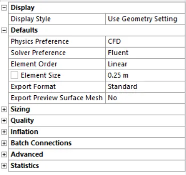
Mesh the 2D model by providing the proper element size(ideally size 0.25 m) and type of the mesh shape (here we want triangular mesh). Also, provide inflation layers (to get better results near the wall) and number of divisions(under mesh sizing) on the cylinder wall to capture the wall boundary nicely(preferably 36 number of divisions).
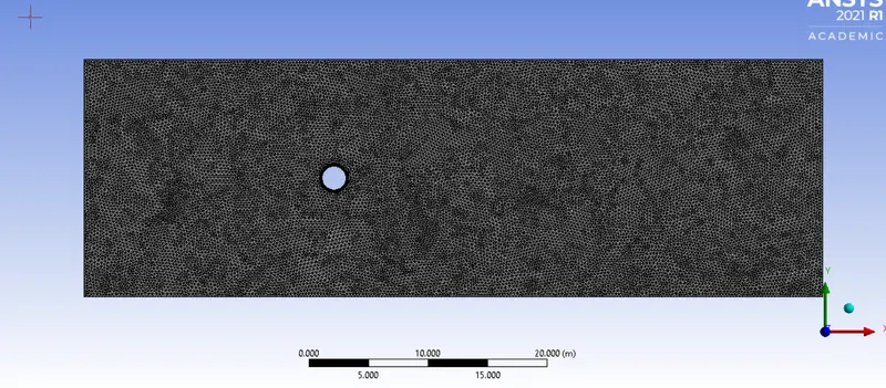
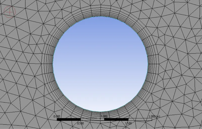
After that, select edges of the geometry and provide boundary names accordingly, “inlet” for the side where the air is supposed to enter, “outlet” for the side where the air will exit, “wall” for cylinder wall and “symmetry” for the boundary condition for the length of the geometry. This will help ANSYS to auto assign some of the boundary conditions while initializing the simulation.
3. Set Up:-
setup the general settings accordingly
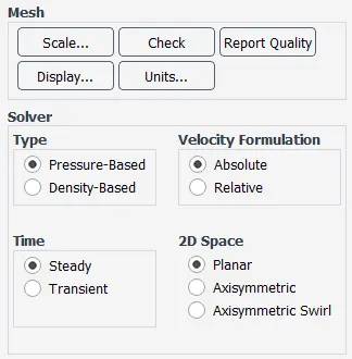
Select laminar flow inside the viscous model.
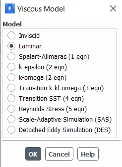
To customize material property for simulation, materials > fluent database > select the material (air) > copy it> rename the name of material to "user material".
Boundary Condition:-
Outlet : gauge pressure = 0 Pa.
wall : no slip condition and stationary wall.
inlet: inlet velocity(m/s)
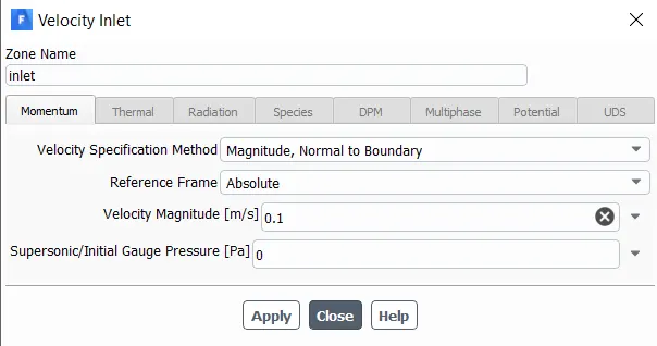
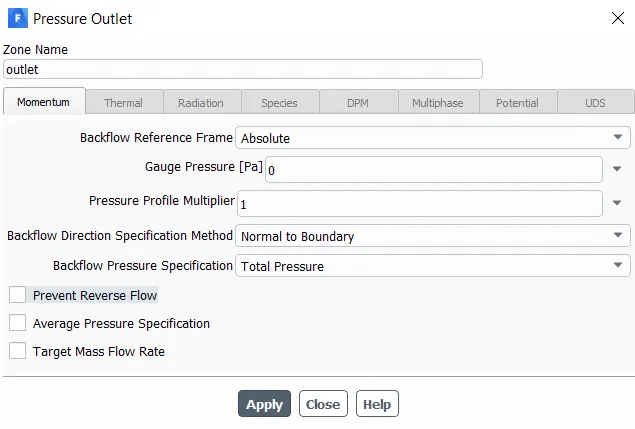
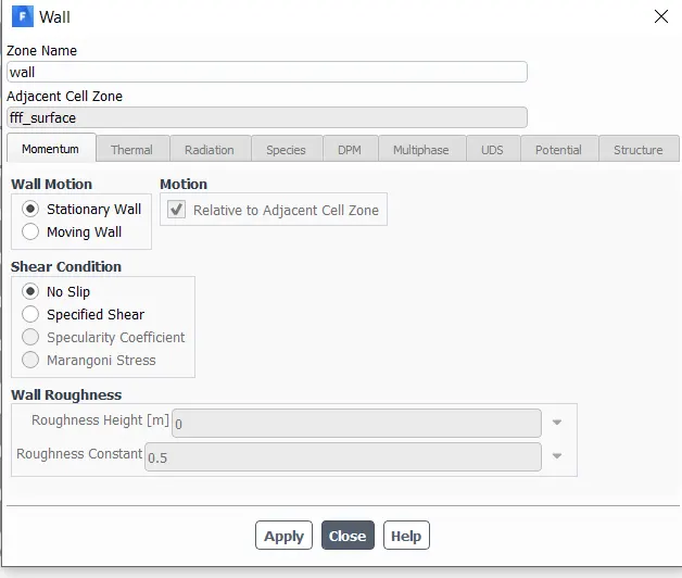
5. Changing the material property:- the next step is to change the material property according to our need so that we can change the Reynolds number by varying either the velocity of the flow of air over the cylinder ,density or viscosity of the fluid. We have used the density of the material, in our case, it is air, as 1 kg/m3 and the viscosity as 0.01803mPa.
6. Adding data points and graphs:- We also need to create that we will be doing. We also need
The coordinates of this point are (8,0) in the x-y axis.
To create the Coefficient of drag and the Coefficient of Lift plots from the simulations plots, and to find the velocity at a particular point(X=8m, Y=0) at a particular distance away from the circle towards the outlet of the domain. we need to use the "definitions" tool and then create these plots and a report for these quantities as well. We then need to study these plots and draw conclusions from them.
7. To calculate strauhall number:- To calculate staruhal no. using ansys fluent, follow the steps below:
1. Go to fluent solver > results > fft analyser > load lift coefficient file > select plot FFT
Here, x axis denotes strauhal number and y axis denotes magnitude.
2. To get the magnitude of strauhal number,
go to results > fft analyser > click on write fft to file > click on write fft.
3. open the file in excel and 1st coloumn denotes the frequncy and 2nd coloumn denotes strauhal number.use the command max and select 2nd row and find the magnitude of strauhal number.
8. Varying inlet velocities to change Re:- We have various cases that we study under this assignment where we vary the Reynolds number by varying the Inlet Velocity. We vary the Reynolds Number from Re= 10,100,1000,10000,100000 by varying the type of solver and the Inlet Velocity according to the Reynolds number for which we are performing the simulation.
OBSERVATIONS:-
Part-1 (steady state vs. transient state simulation at Re=100) :-
Steady state simulation results:-
average vortex velocity
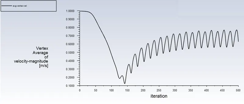
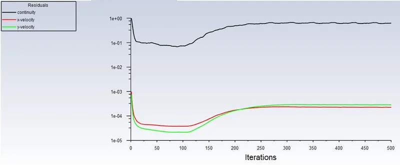
convergence reached around iteration number=350
residuals
coefficient of lift
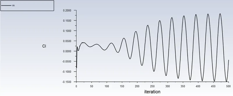
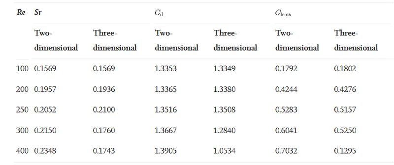
Cl=0.175
error=1.1%
coefficient of drag
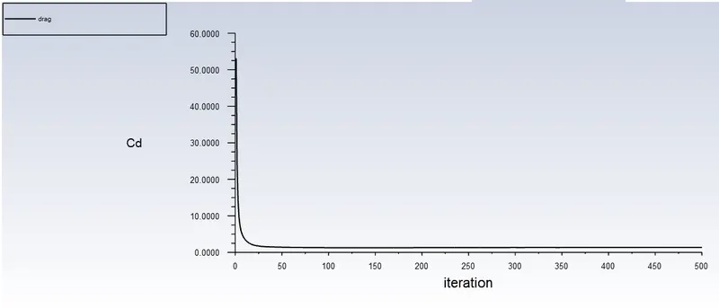
Cd=1.35
error in %= 1.5%
Strouhal Number
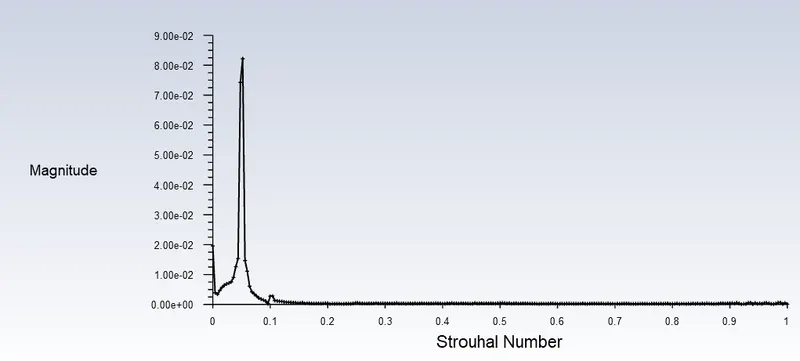
Strouhal no.=0.05
pressure and velocity contours
velocity
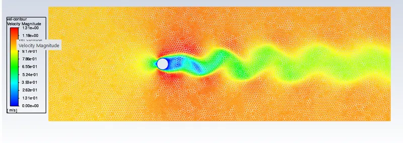
pressure
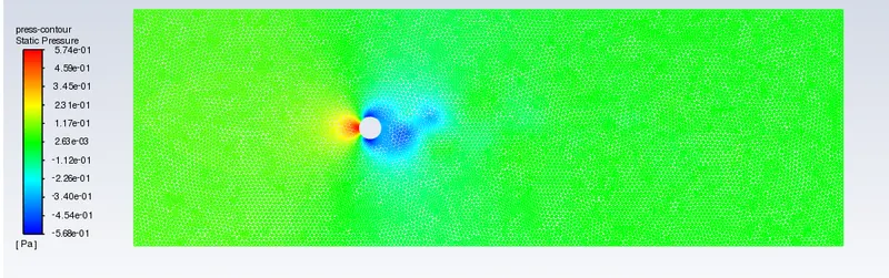
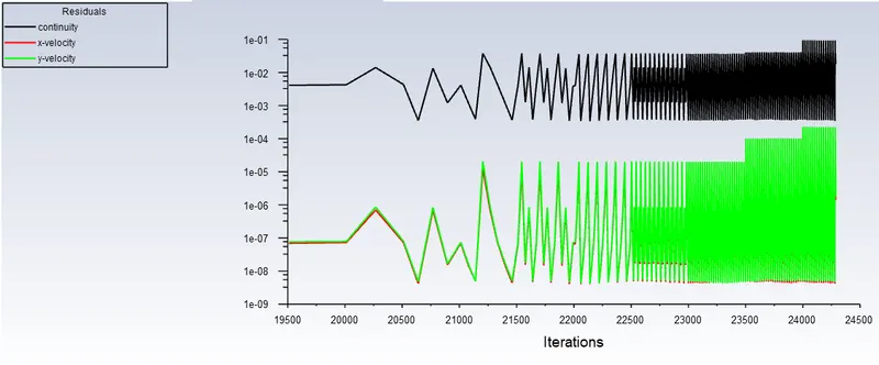
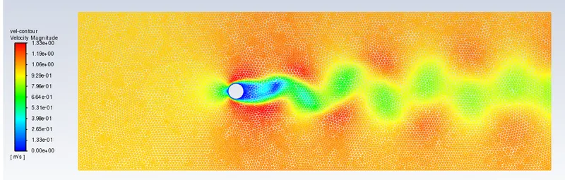
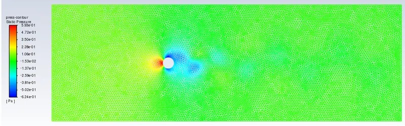
Transient state simulation results:-
average vortex velocity
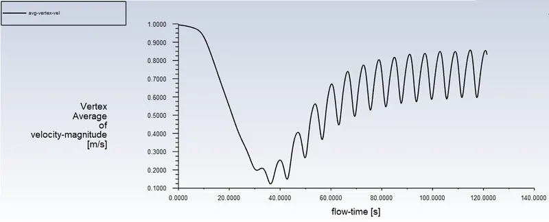
convergence reached around flow-time=100
residuals
coefficient of lift
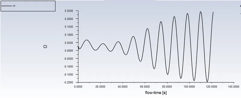
Cl=0.18
error=4%
coefficient of drag
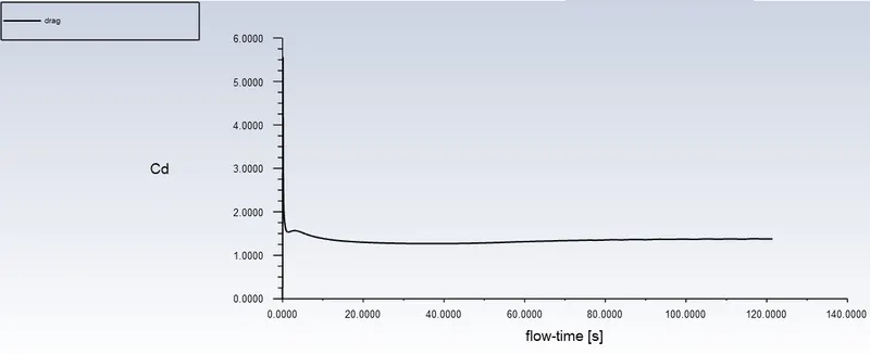
Cd=1.37
error=3%
Strouhal Number
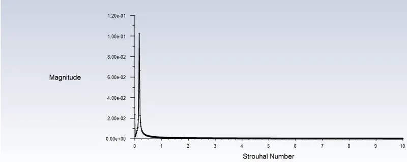
Strouhal no.=0.02
pressure and velocity contours
velocity
pressure
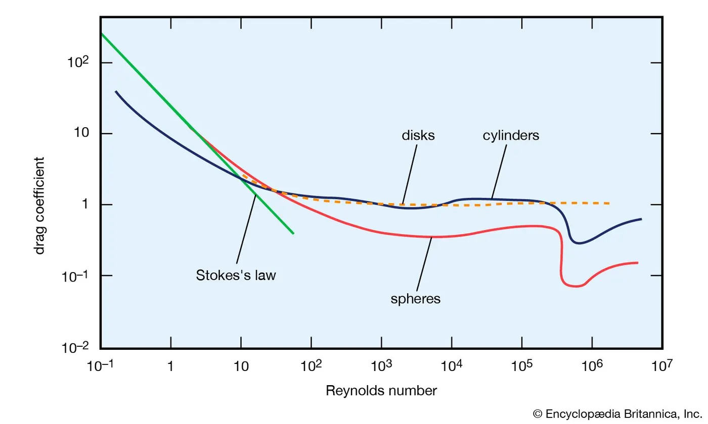
Note: error in lift and drag coefficients were calculated at Re=100, from reference values from picture below
Part-2 (steady state simulation at Re=10,100,1000,10000,100000) :-
Re=10
average vortex velocity
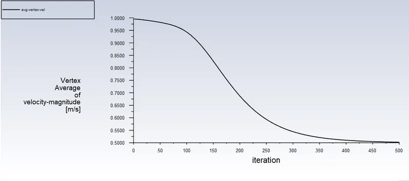
convergence reached around iteration number=490-500
residuals
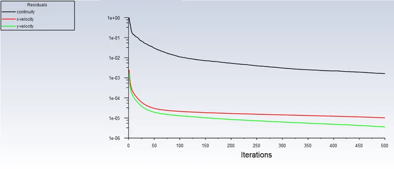
coefficient of lift
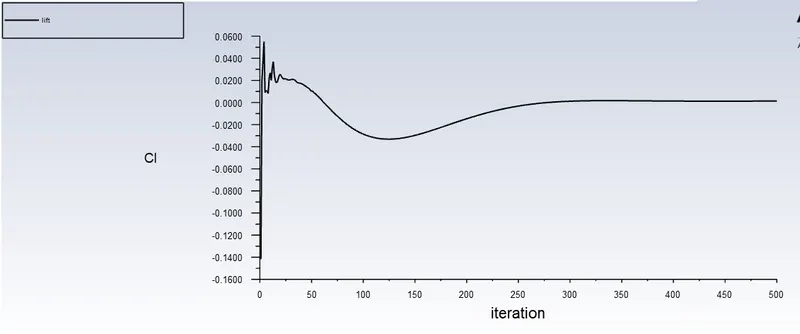
Cl=0.0013
coefficient of drag
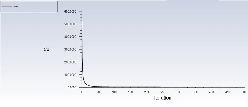
Cd=3.322
pressure and velocity contours
velocity
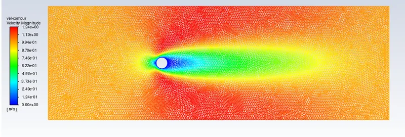
pressure
Observation at Re=10 and 100
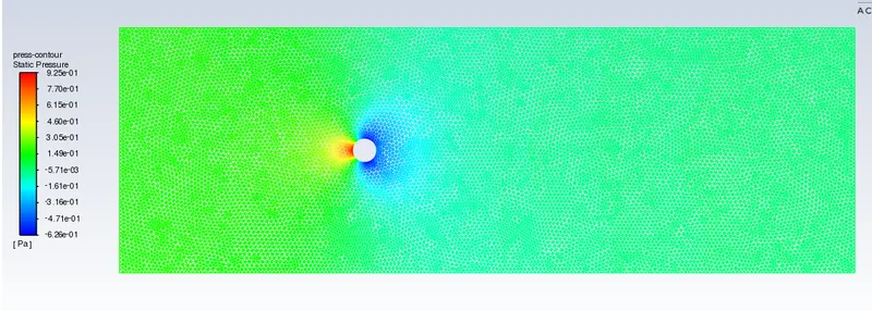
At Re = 10, the flow is still a bit laminar but a visible separated (wake) flow region appears in the rear of the cylinder. Therefore the flow no longer exhibits the fore and aft symmetry, albeit it is still symmetric about the mid-plane. As the value of the Reynolds number is increased further, the wake region is characterized by a pair of counter-rotating vortices that remain attached
Also at Re = 100, from case 1 steady state simulation, the wake becomes unstable (initially originating from the downstream end) and the viscous forces are no longer sufficient to overcome these disturbances. The instability grows further with the increasing Reynolds number. the flow is still laminar and two-dimensional. However, one needs to solve the time-dependent momentum equations to resolve the vortex-shedding characteristics in this flow regime.
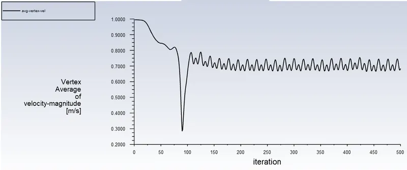
Re=1000
average vortex velocity
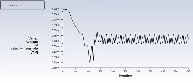
convergence reached around iteration number=160-170
residuals
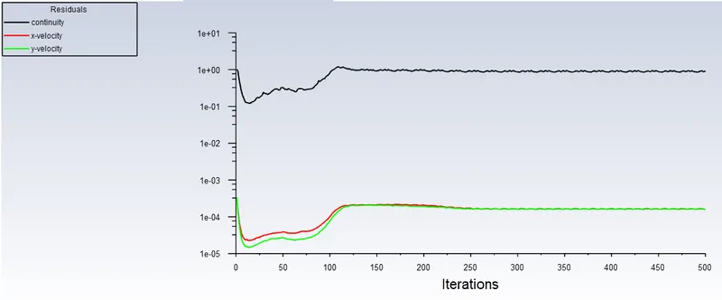
coefficient of lift
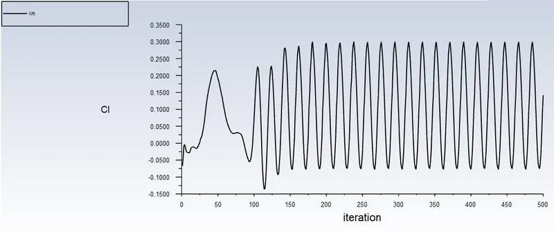
Cl=0.29
coefficient of drag
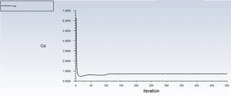
Cd=0.73
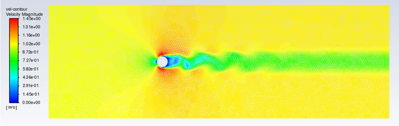
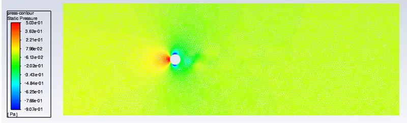
pressure and velocity contours
velocity
pressure
Re=10,000
average vortex velocity
convergence reached around iteration number=200
residuals
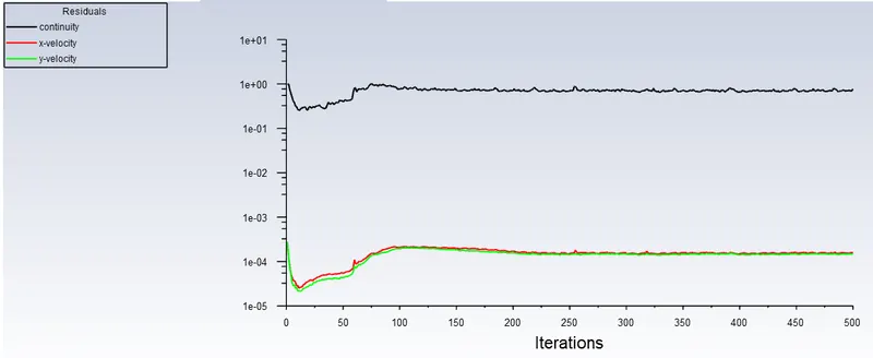
coefficient of lift
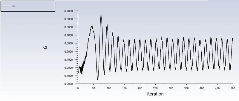
Cl=0.375
coefficient of drag
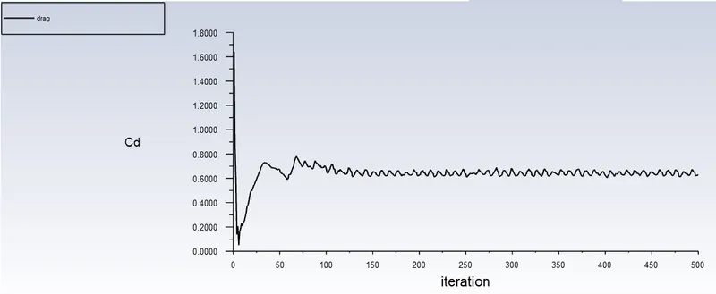
Cd=0.65
pressure and velocity contours
velocity
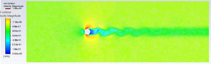
pressure
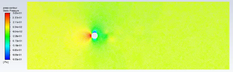
Re=100,000
average vortex velocity
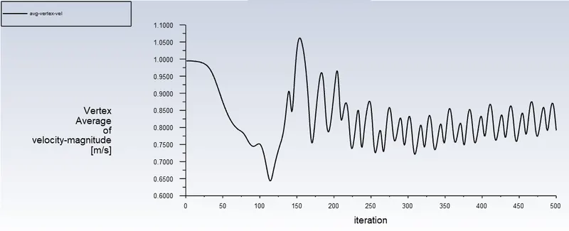
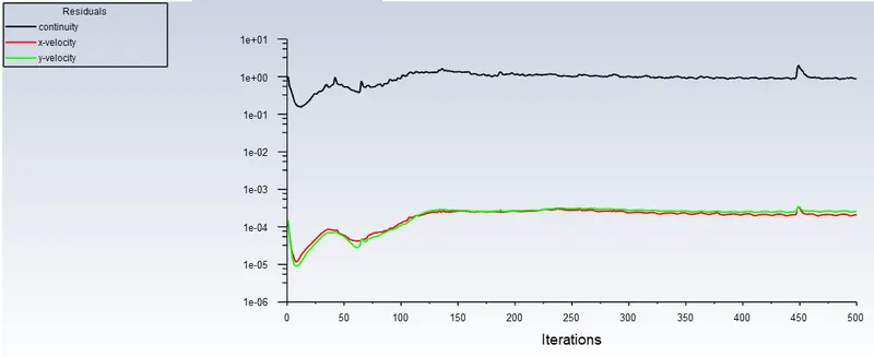
convergence reached around iteration number=400
residuals
coefficient of lift
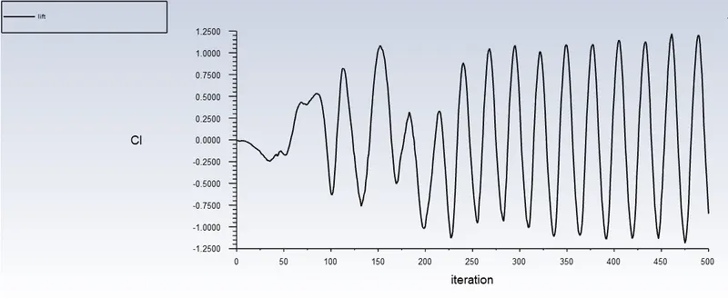
Cl=1.19
coefficient of drag
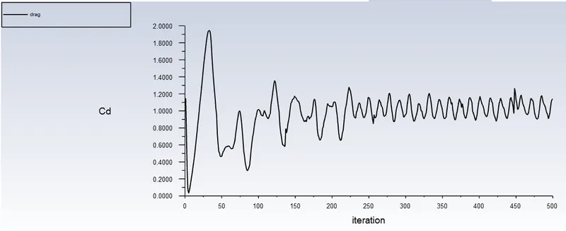
Cd=1.13
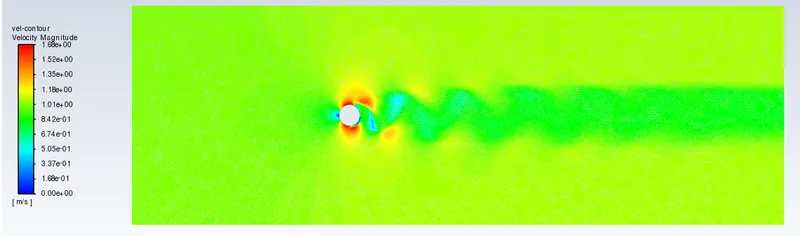
pressure and velocity contours
velocity
pressure
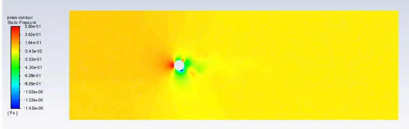
Observation from Re=1000 to Re=100,000
Further increase in the value of the Reynolds number induces increased levels of turbulence in the boundary layer and wake region.
Cd decreases till Re=10,000 then reaches almost the same level, as the Cd in Re=100, when the Re=100,000 (Cd=1.13). explanation for this is given in results section.
note:
As we discussed above, in a vortex street simulation we most probably never get our results fully converged. therefore, we need to use the alternate option to see our results are converged or not, so if we notice the velocity results at the monitor point behind the cylinder, there is a constant velocity after certain number of iterations iterations. Hence In the vortex shedding charts, all the results at constant frequency repeating themselves. therefore, we can consider at those points as our converged results.
Results:-
effect of Reynolds number on the coefficient of drag and lift:-
The above plots exhibit, drag plots for Reynolds number 10,100,1000,10000, and 100000. If the Reynolds Number is large, the viscosity effect is small.
In practical values the inertia or density forces dominate, and the parasite drag increases with the square of the velocity. However, although the viscosity is unimportant, it may still affect the very thin boundary layer, leading to the creation of turbulent flow. Thus the importance of the Reynolds Number is that it tells us the type of flow we can expect. It tells you whether you can hope for having laminar flow over the wing and other parts of your airplane. A low Reynolds Number gives laminar flow while a high Reynolds Number gives turbulent flow.
For both a laminar and a turbulent boundary layer increasing Reynolds Number gives lower skin friction drag and then skin friction increases at Re=100,000 till almost the same value as Re=100(refer the plot below). However, because of the higher energy loss in the boundary layer, a turbulent layer always has higher skin friction drag.
As depicted in the Cl plots, the lift is also an oscillating entity, and its oscillation with the same frequency after a particular iteration for each plot. one can observe that the frequency and the oscillation increase with rising in Reynold's number.
it can also be observed that the average lift value was nearly zero for the low Re number but it raises to a positive value with an increase in Reynold's number.
hence the simulation over the cylinder pipe was carried out.
References:-
1) Numerical simulation of laminar flow past a circular cylinder - ScienceDirect
2) Reynolds number - Wikipedia