Week 2 - Flow over a Cylinder.

 AIM:

To simulate the flow over a cylinder and explain the phenomenon of Karman vortex street. 

GIVEN DATA:

PART-I

1. Simulate the flow with the steady and unsteady case and calculate the Strouhal Number for Re= 100. 

PART-II

1. Calculate the coefficient of drag and lift over a cylinder by setting the Reynolds number to 10,100,1000,10000 & 100000. (Run with steady solver)
2. Discuss the effect of the Reynolds number on the coefficient of drag. [ Results should be validated with any standard literature and error should be within 5 %]

Procedure:

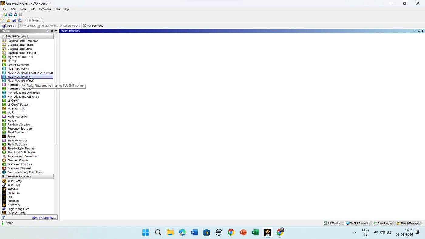
1. Open -----> ANSYS Workbench -----> Flid Fow(Fluent)

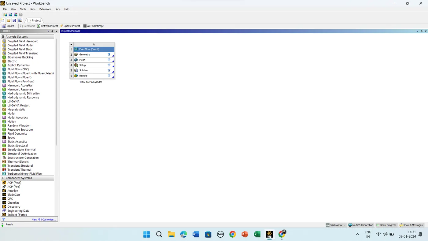
2. Flow over a cylinder double click on the Geomentry

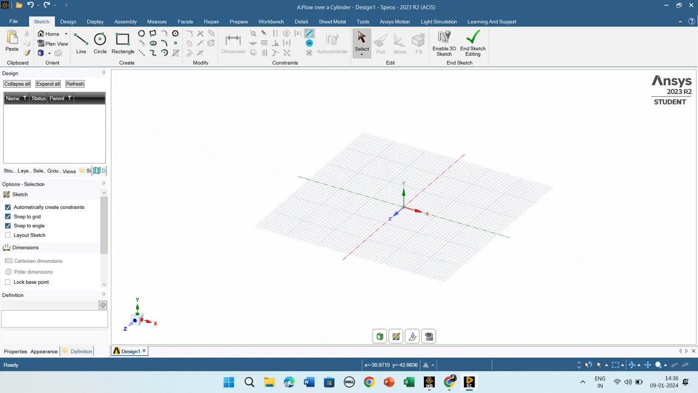
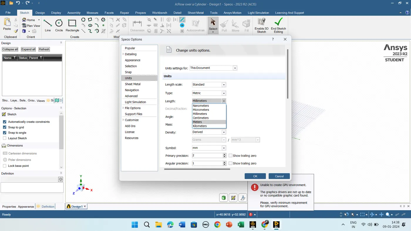
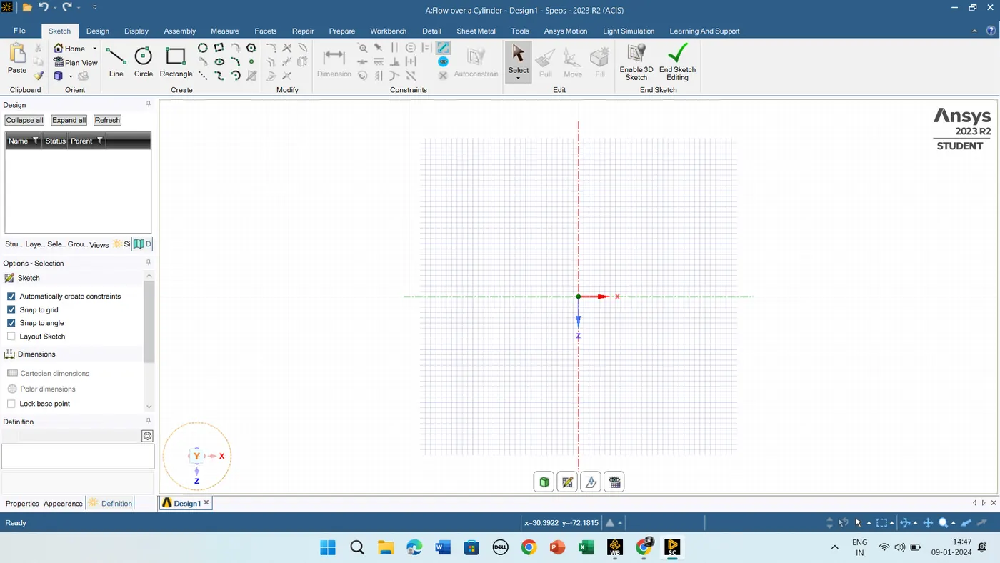
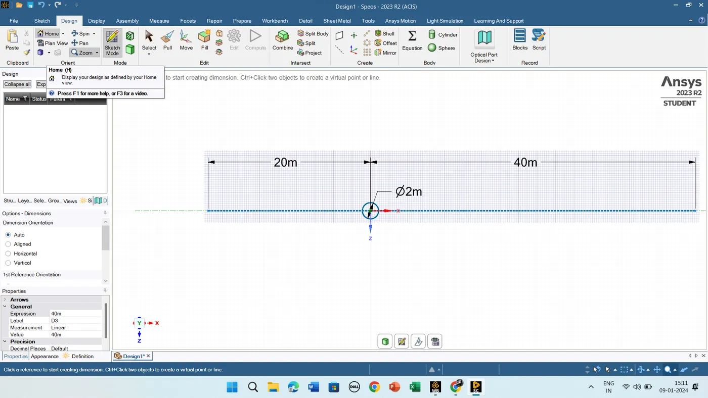
3. Double click on the Geometry to open the space claim, Space Claim OPtion ----> Units ----> Meters ----> Ok. Click on the Y axis and start to sketch.

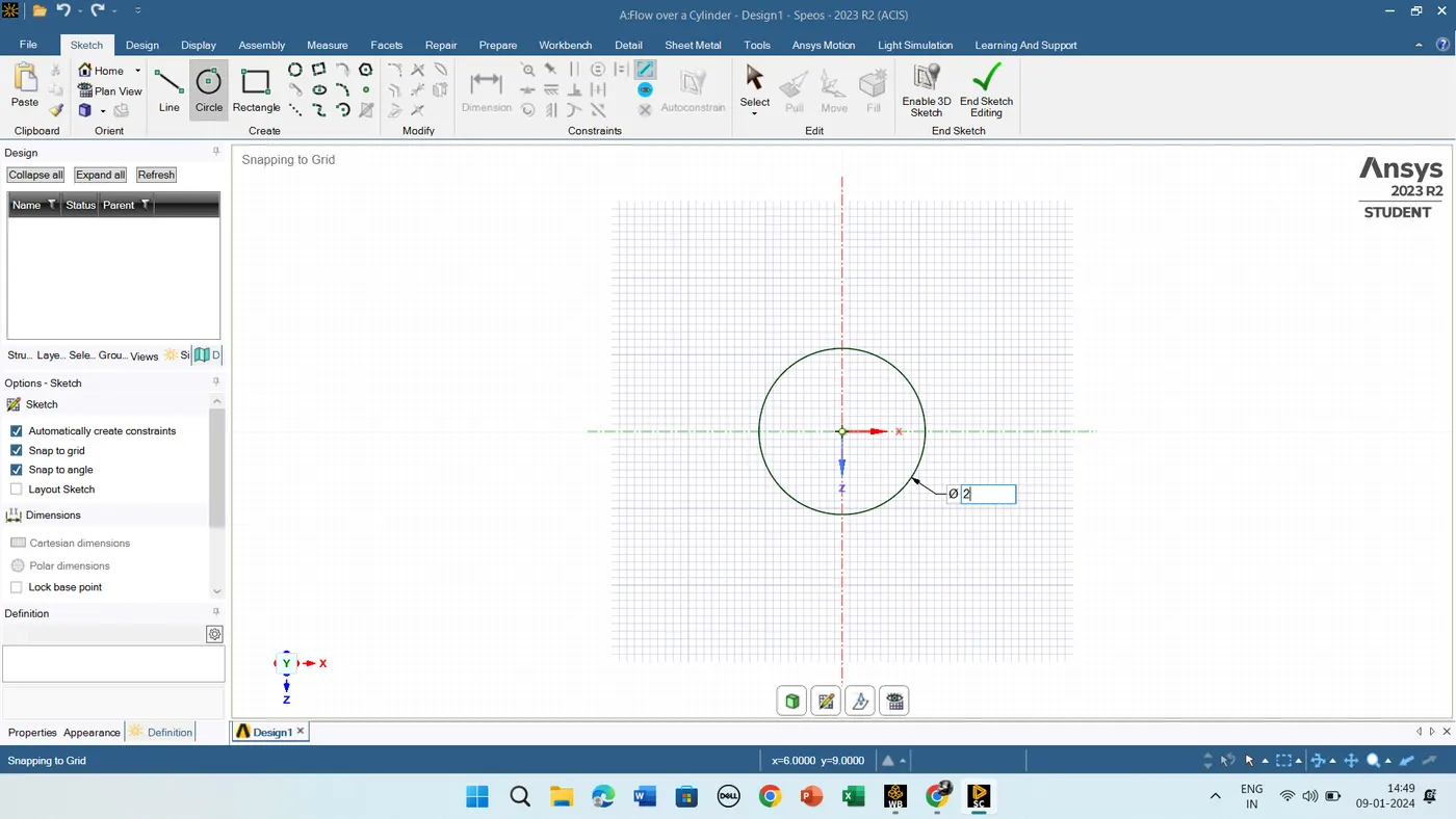
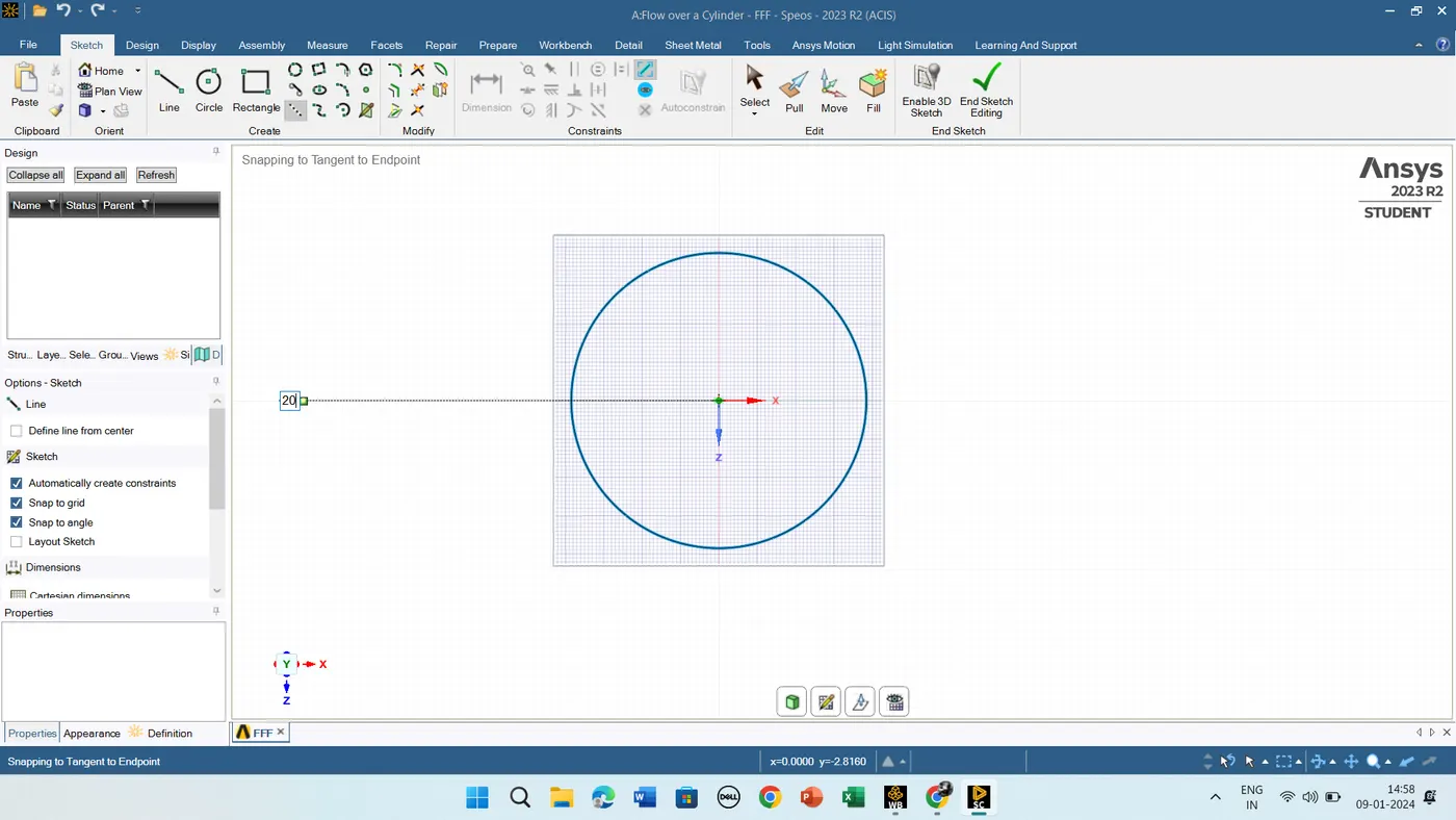
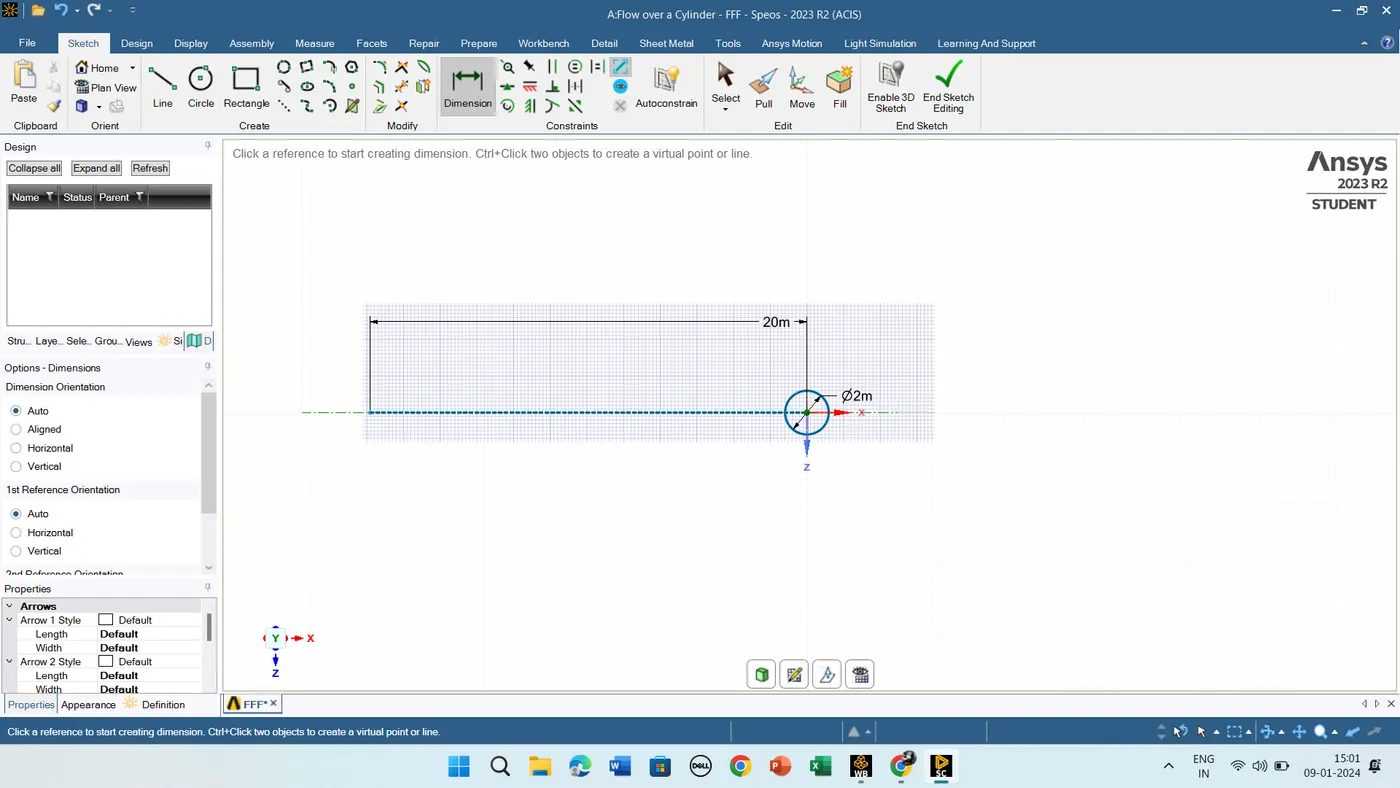
4. Select the Circle ----> Diameter - 2 meters. To create a computational domain click the constructive line and select the centre of the circle draw the line ten times of the Diameter 10 X 2 m = 20 m and to the right draw 40 m (20D).

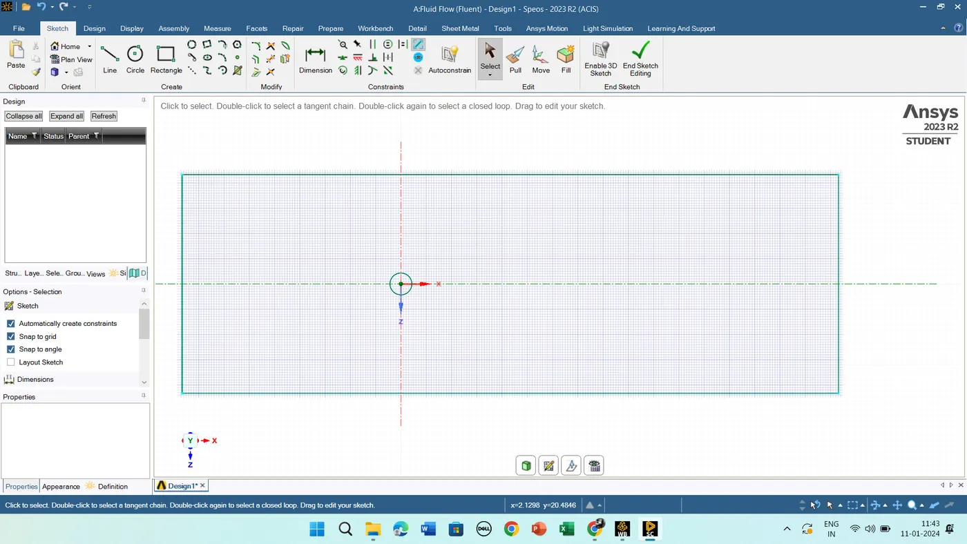
5. Draw the rectangle. 

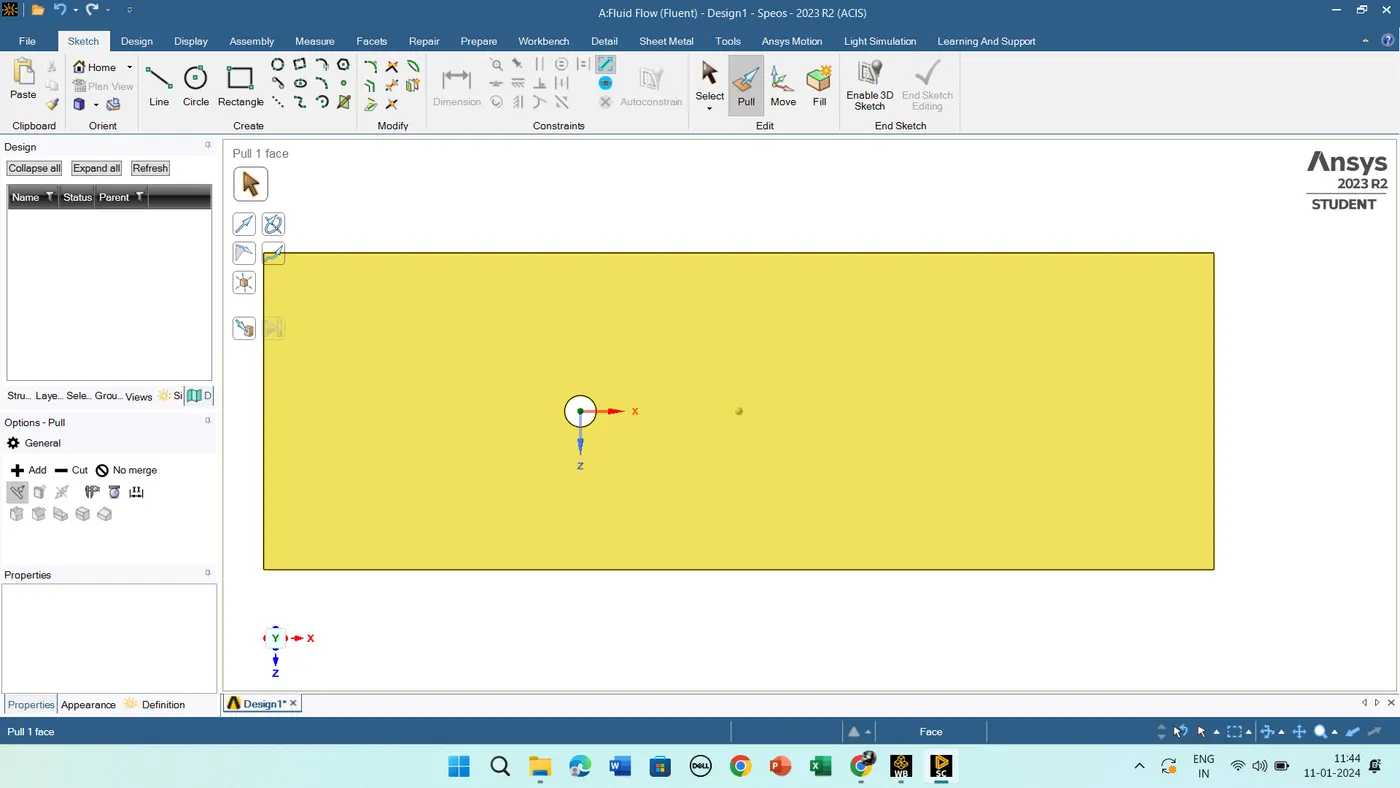
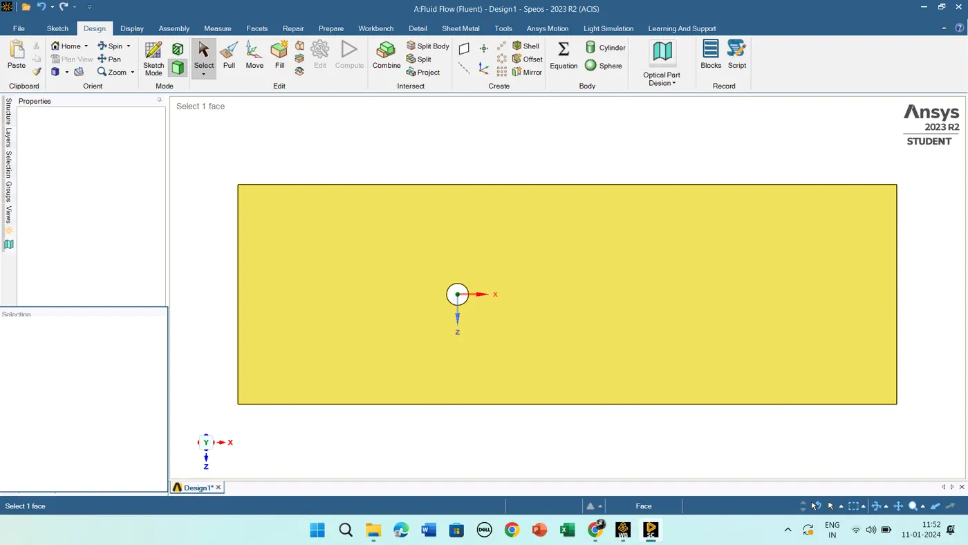
6. Use the pull tool to make a surface 

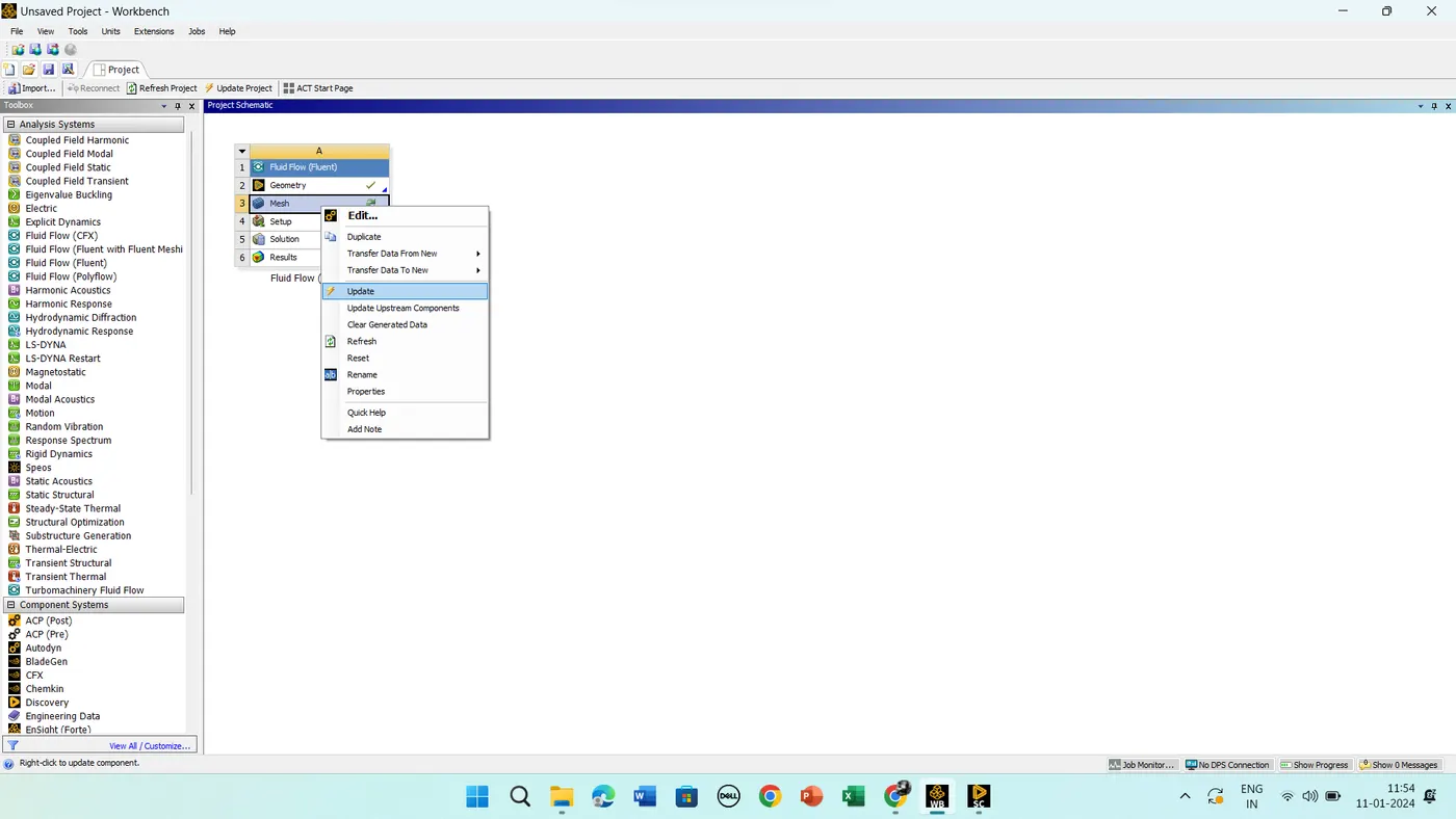
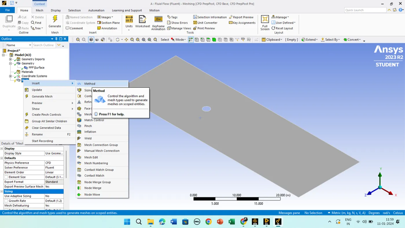
7. Right-click on the Mesh ----> Update and Double-click on the Mesh.

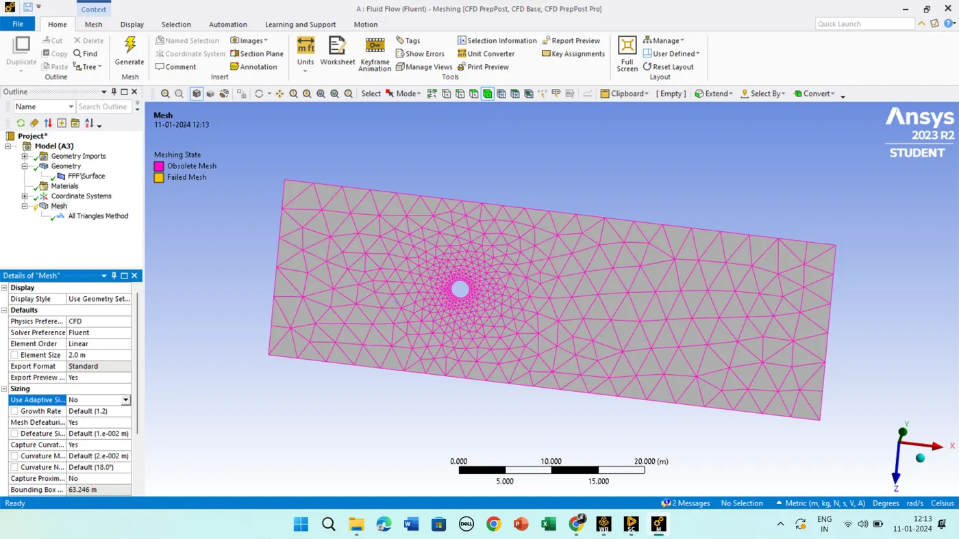
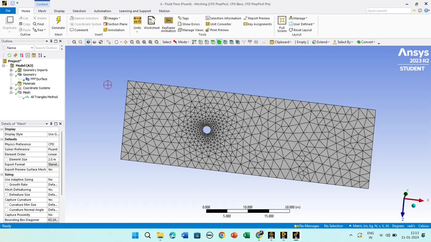
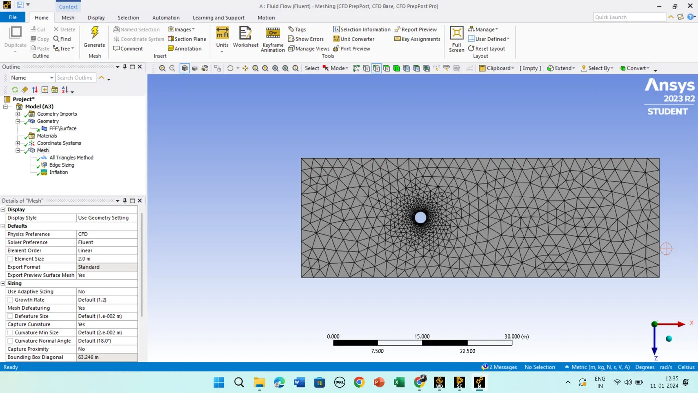
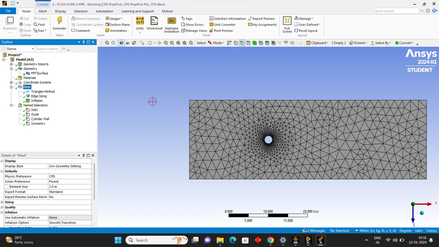
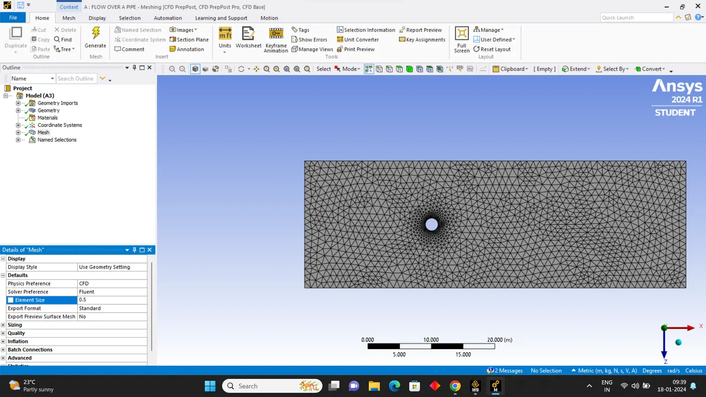
Methods -----> Automatic Method ----> Face ----> Select the Trias ------> Mesh will be generated. Element Size 2mm ----> Generate Mesh. Go to ANSYS Fluent ---> Update the mesh.

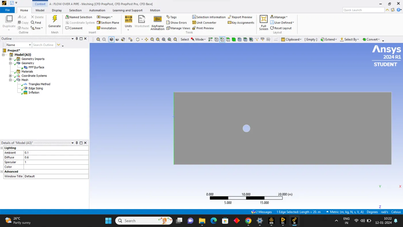
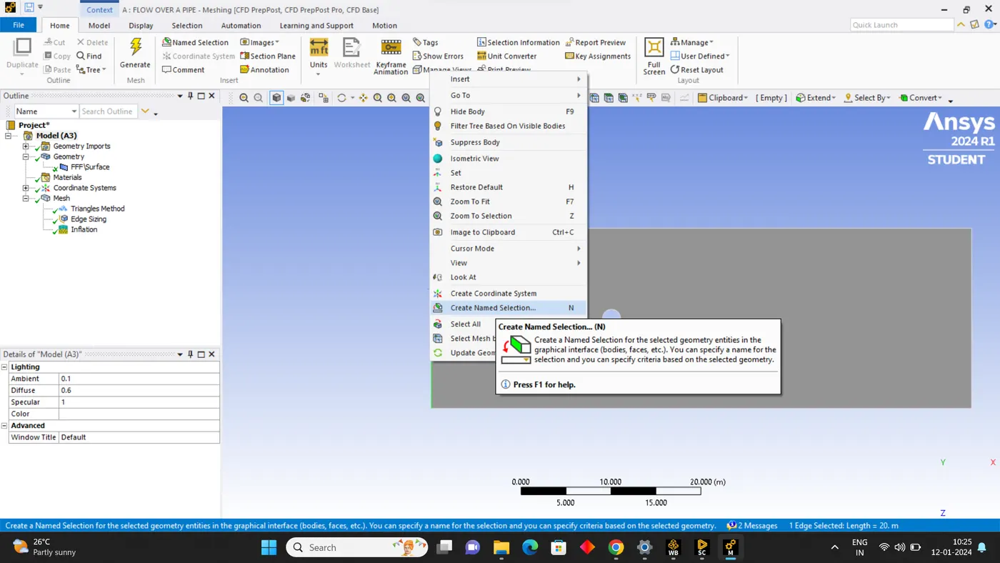
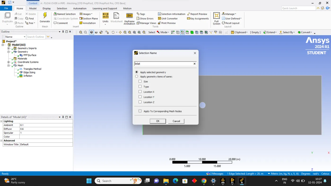
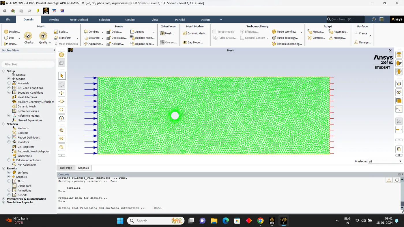
Mesh ----> Select Edge mode Click on the Inlet and right-click ----> Create Named Selection ---> Inlet same do it for outlet, Cylinder wall, and symmetry.

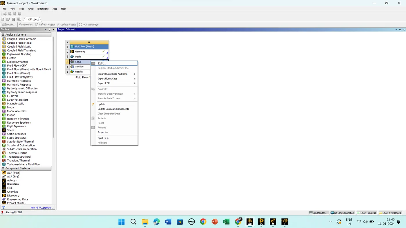
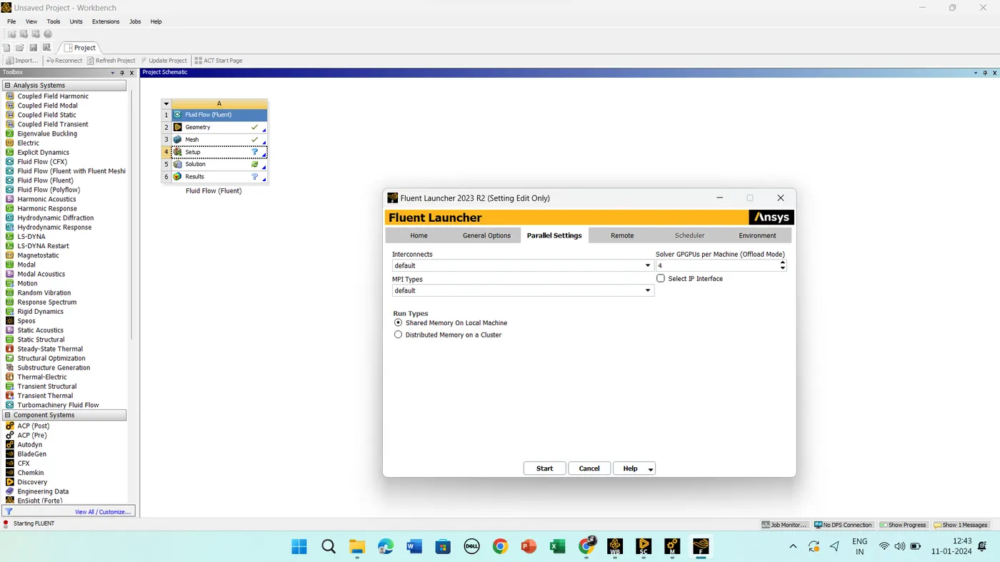
8. Setup -----> Update ----> Edit ----> Select the Double Penetration and run in 4 cores -----> Start.

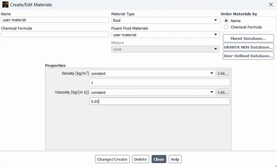
9. By changing the material property in the physics we can able to achieve the vertex shedding for the steady 

10. Post Processing                            

 

  ----

1.

2.

GEOMENTRY

3.

4.

5.

 

6. 

7. 

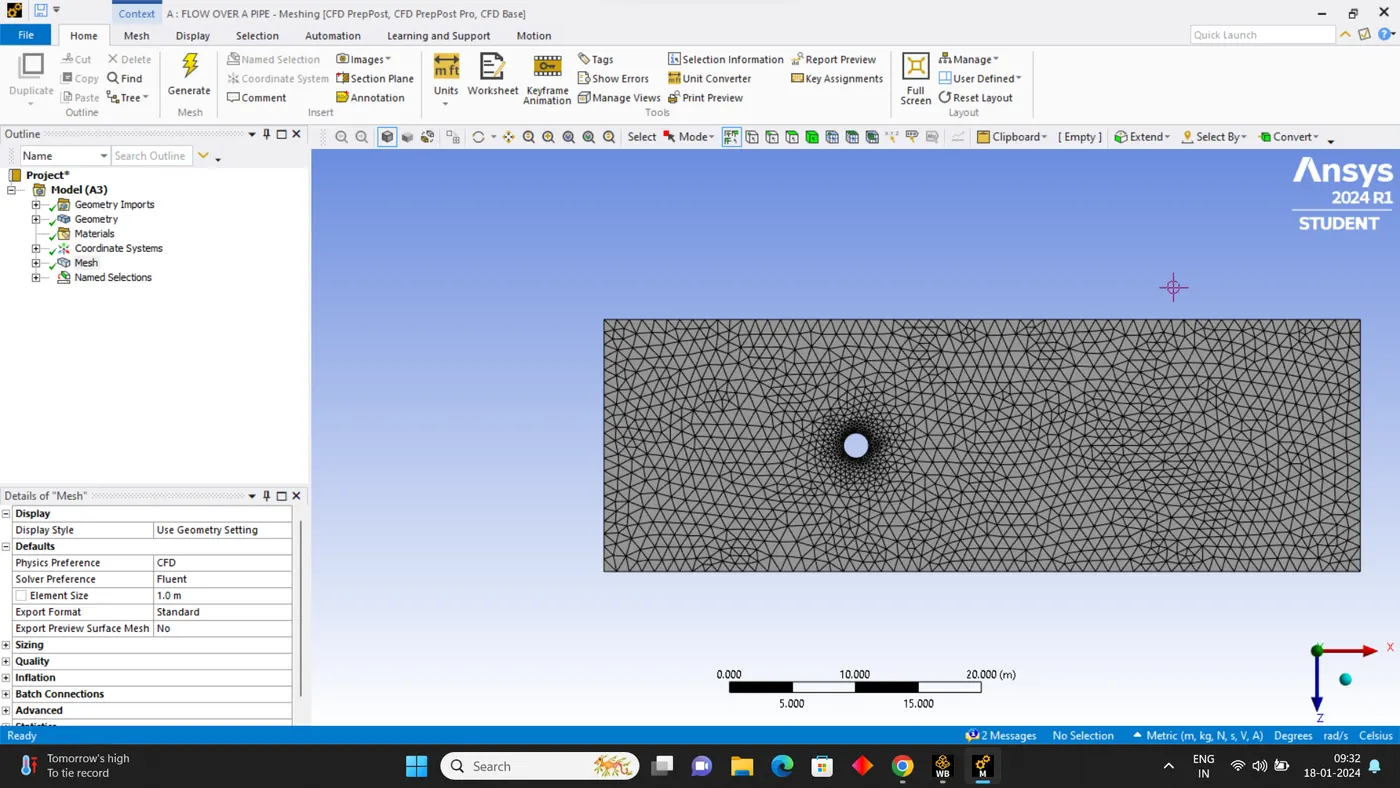
MESHING:

8.

 

 

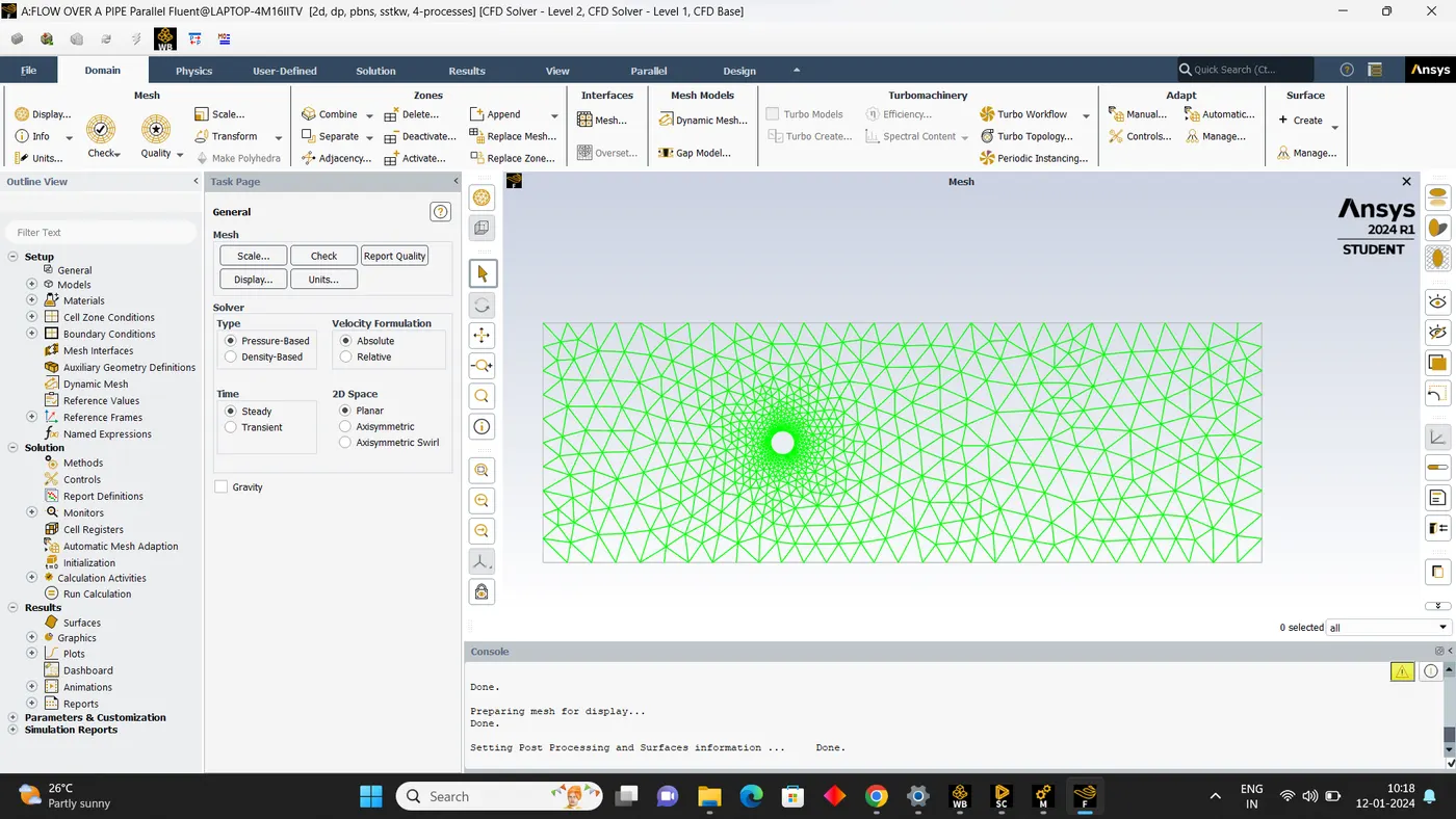
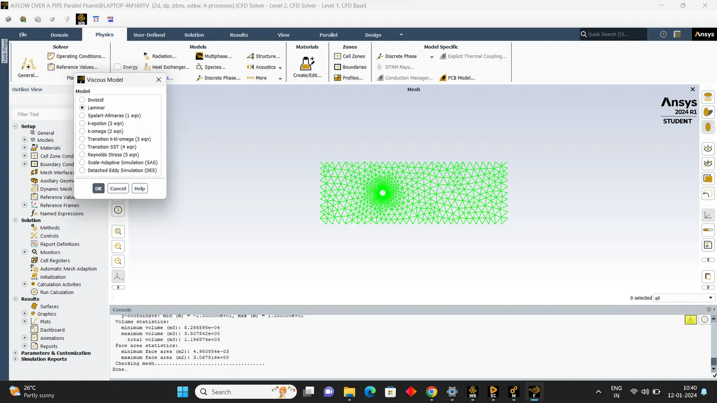
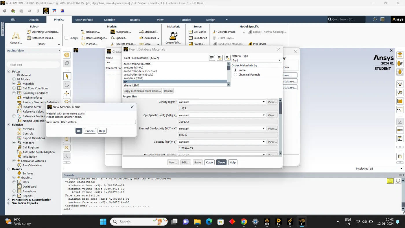
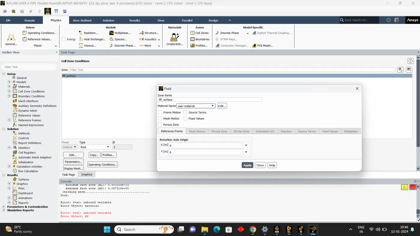
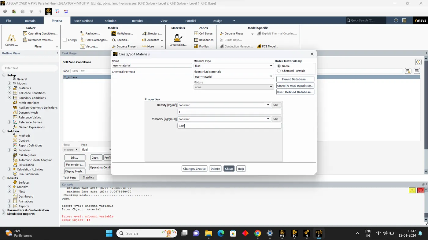
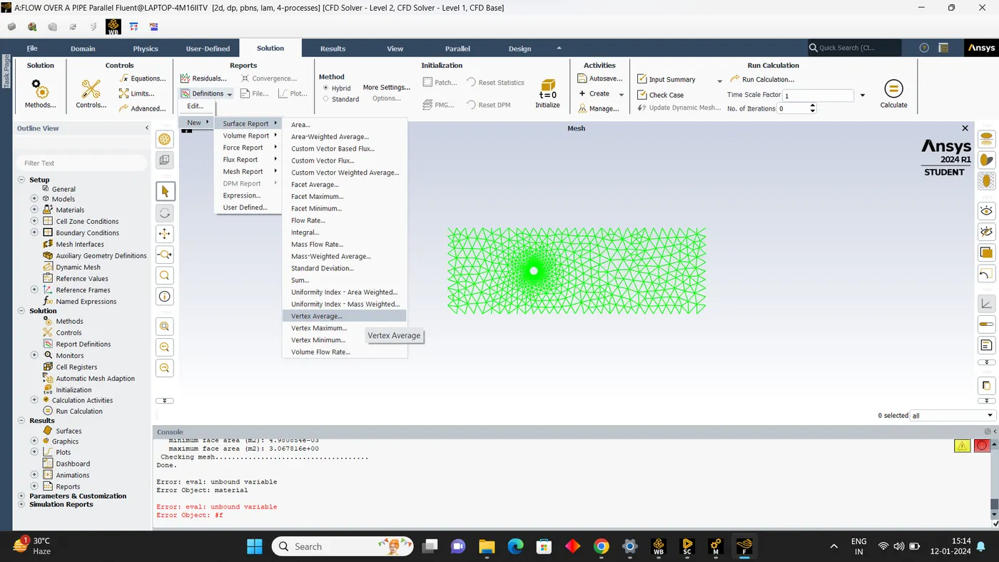
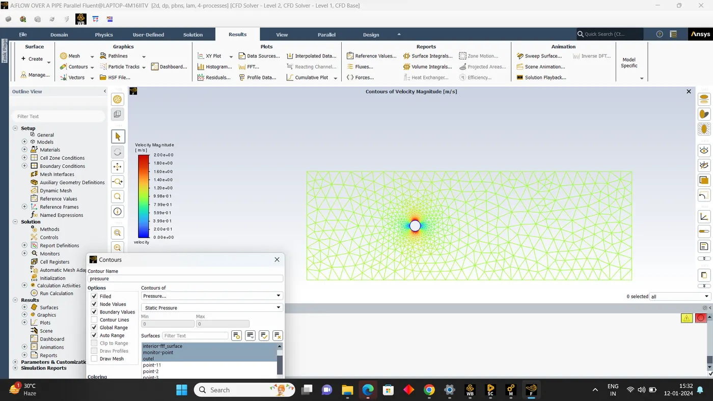
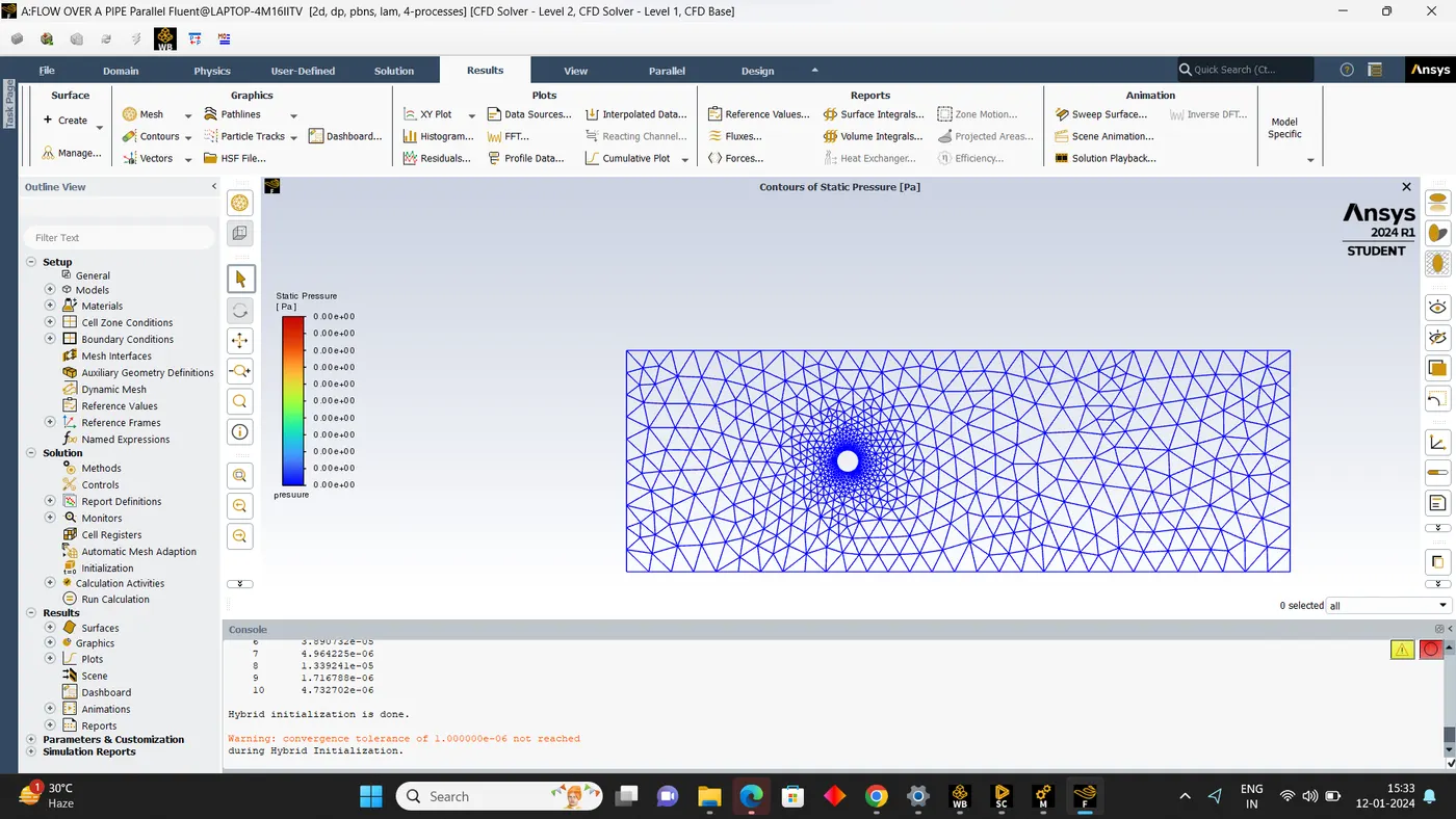
POST PROCESSING

 9.

PART-I

STEADY

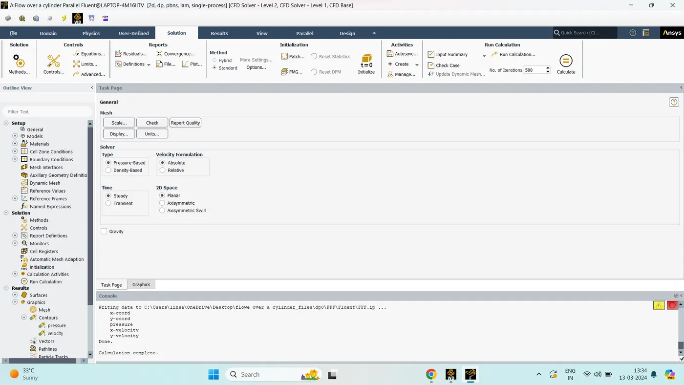
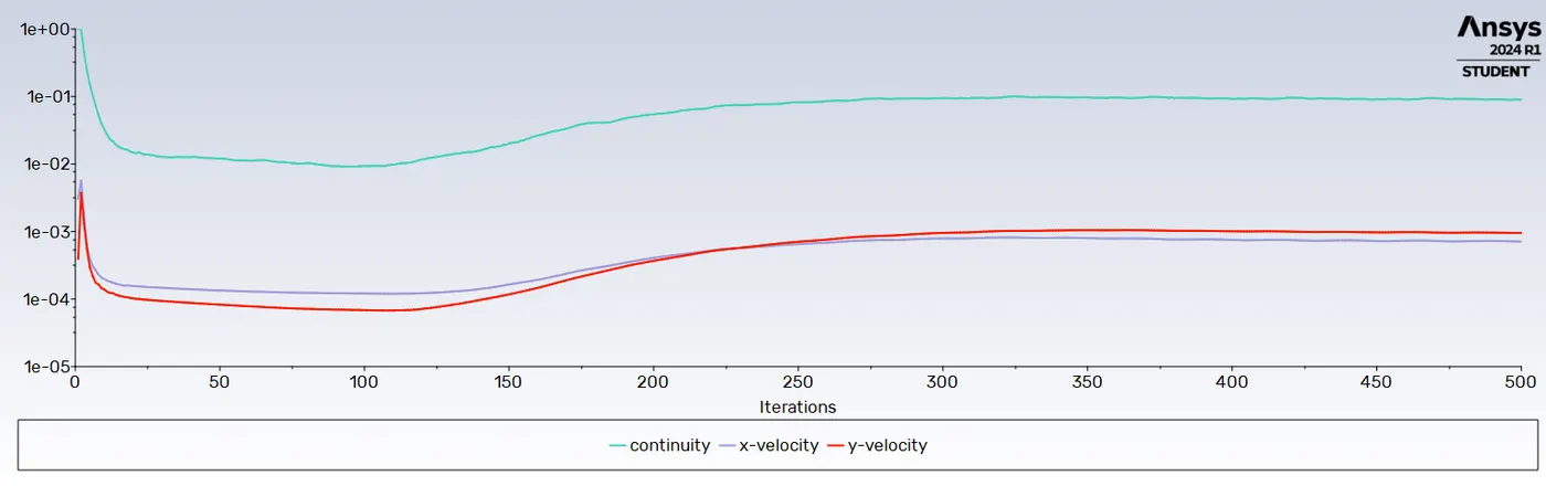
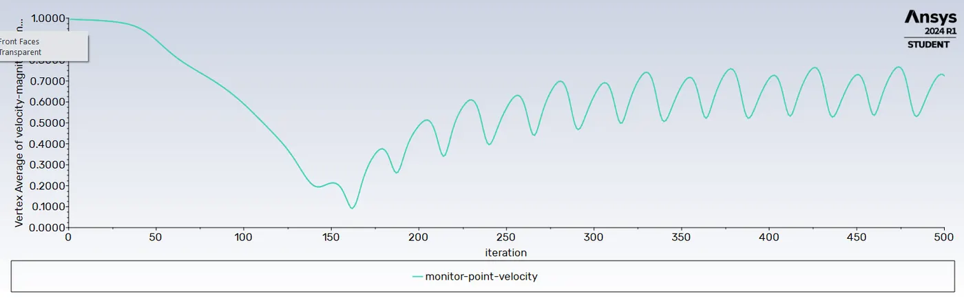
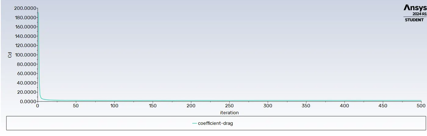
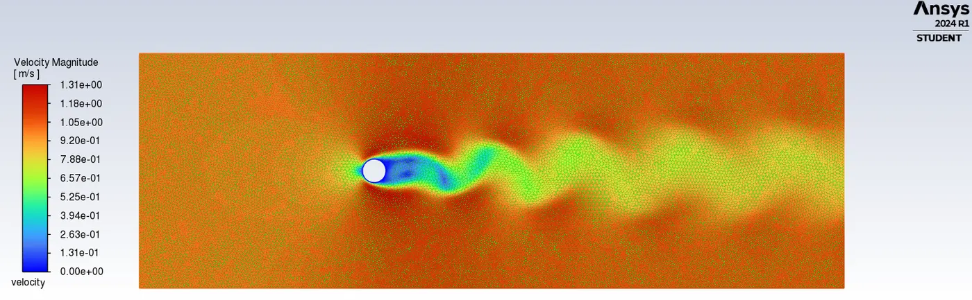
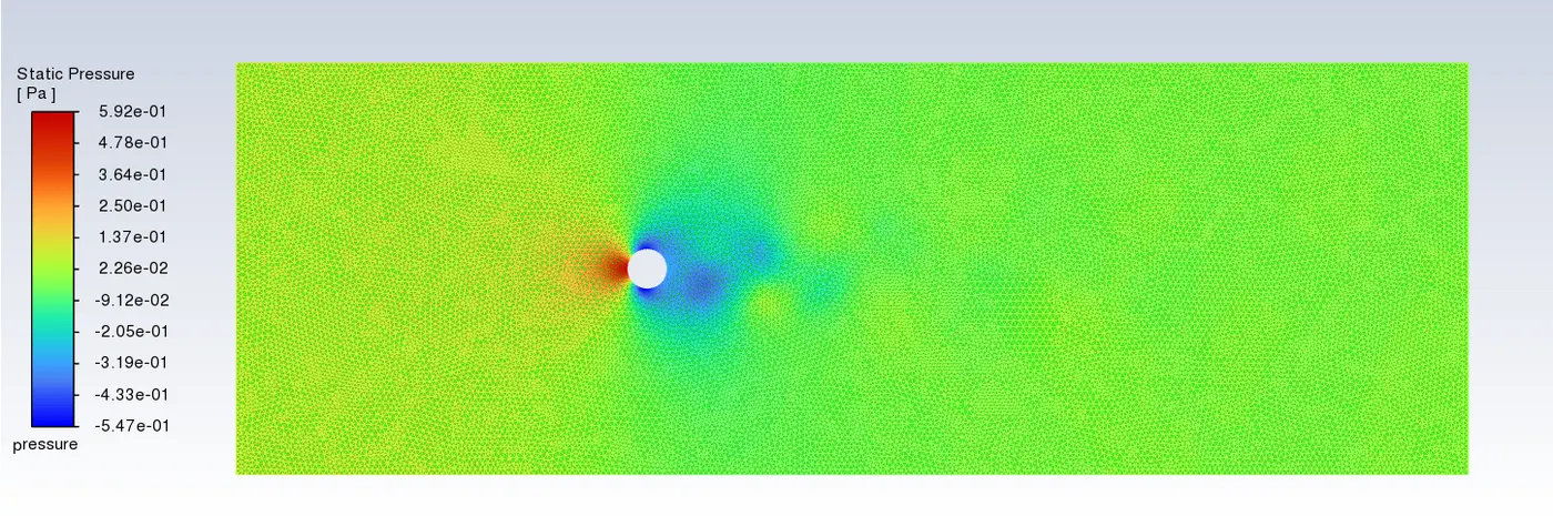
Steady-State Analysis:

Steady-state analysis assumes that the flow variables (velocity, pressure, temperature, etc.) do not change with time. The system has reached a stable equilibrium.

Time-Independence:

In steady-state simulations, all time derivatives are set to zero, simplifying the governing equations.

Convergence:

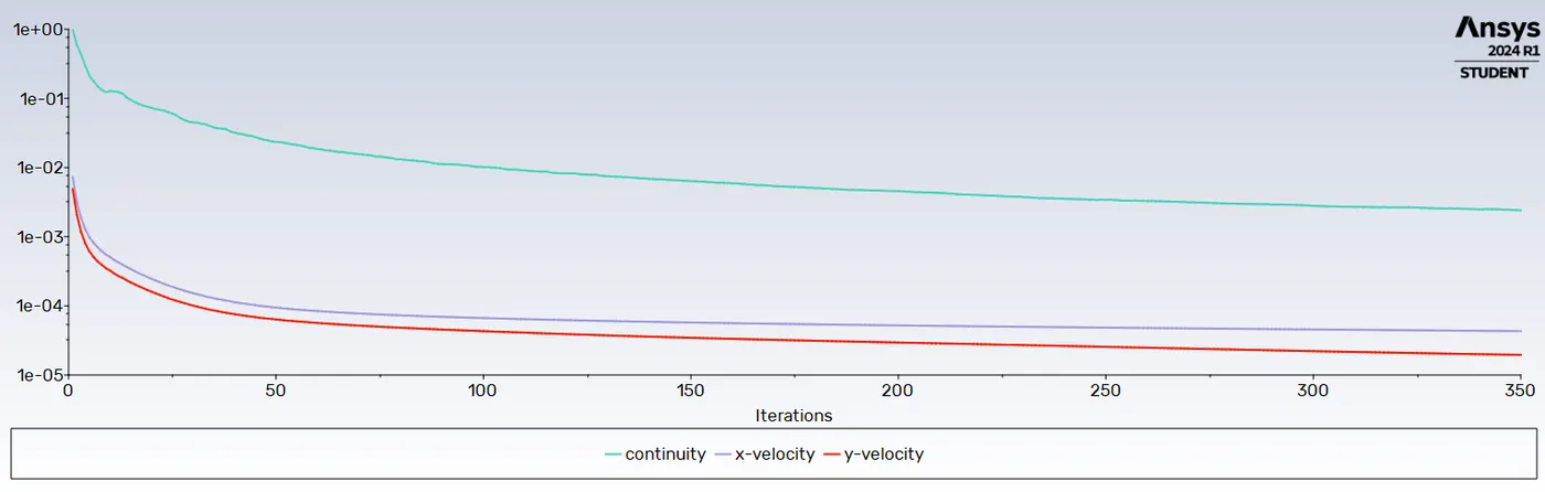
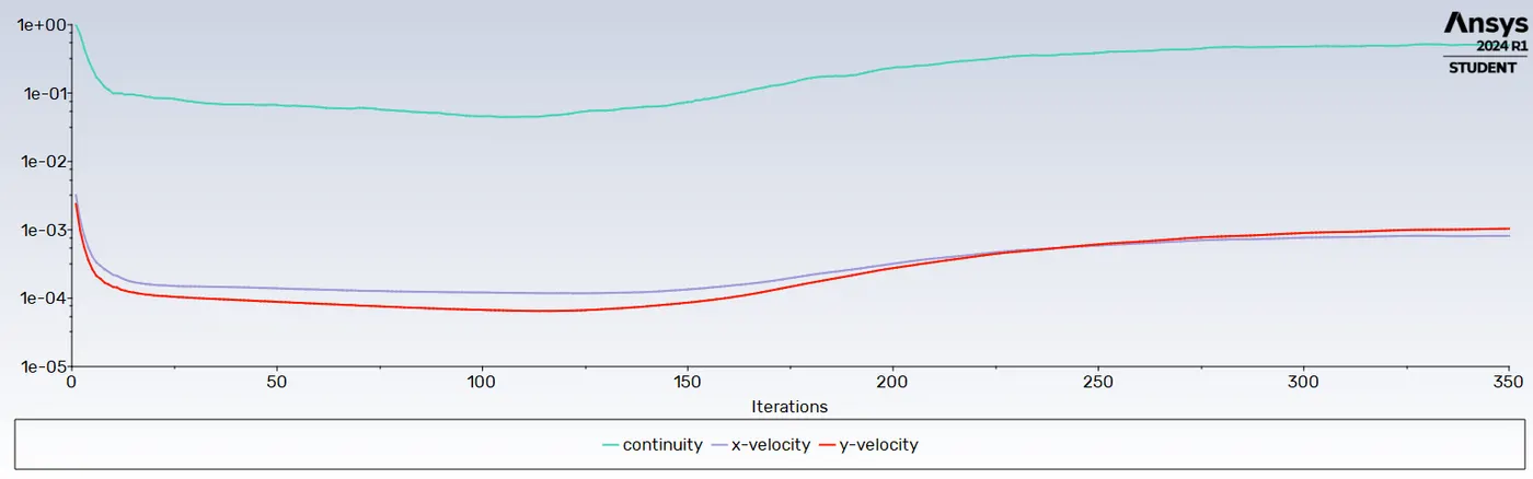
Convergence criteria focus on reaching a stable solution where the solution does not change significantly between iterations.

Applications:

Commonly used for scenarios where the flow conditions do not change over time, such as incompressible fluid flow through pipes, heat exchangers, and some aerodynamic applications.

Advantages:

Faster computation compared to transient simulations.

Requires less computational resources.

Limitations:

Not suitable for scenarios where time-dependent effects are critical.

May not capture dynamic behavior or transient events.

UNSTEADY 

10.

 

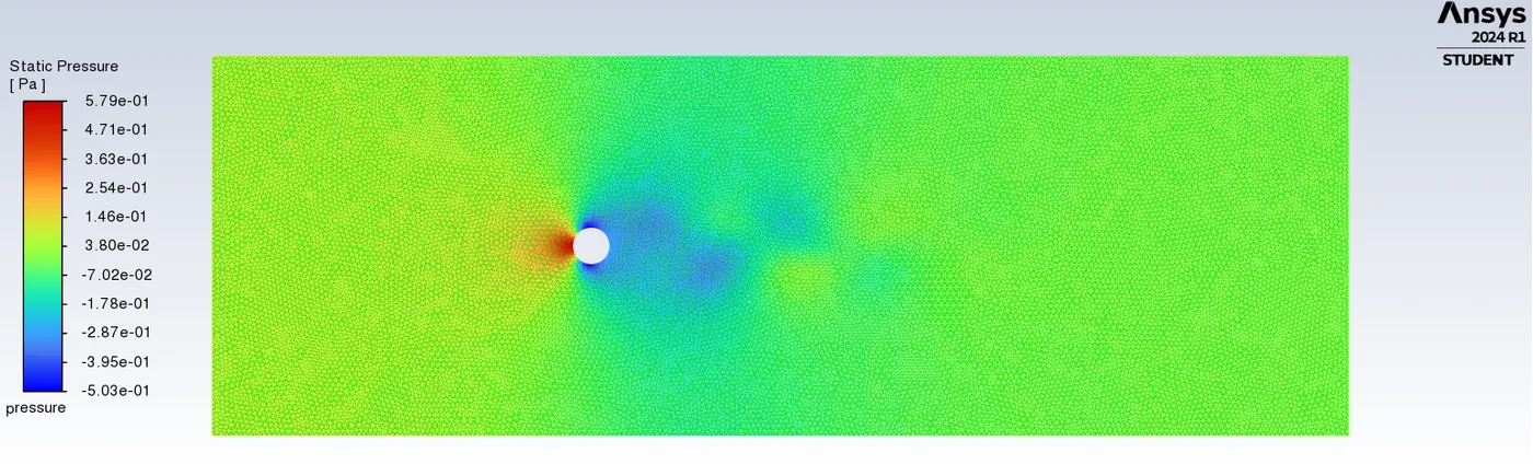
Transient Analysis:

Definition:

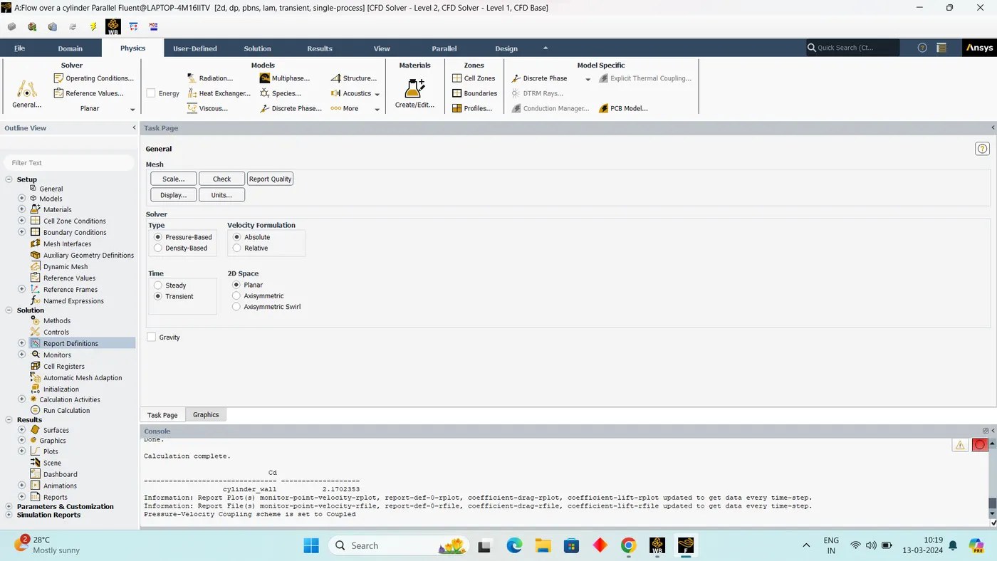
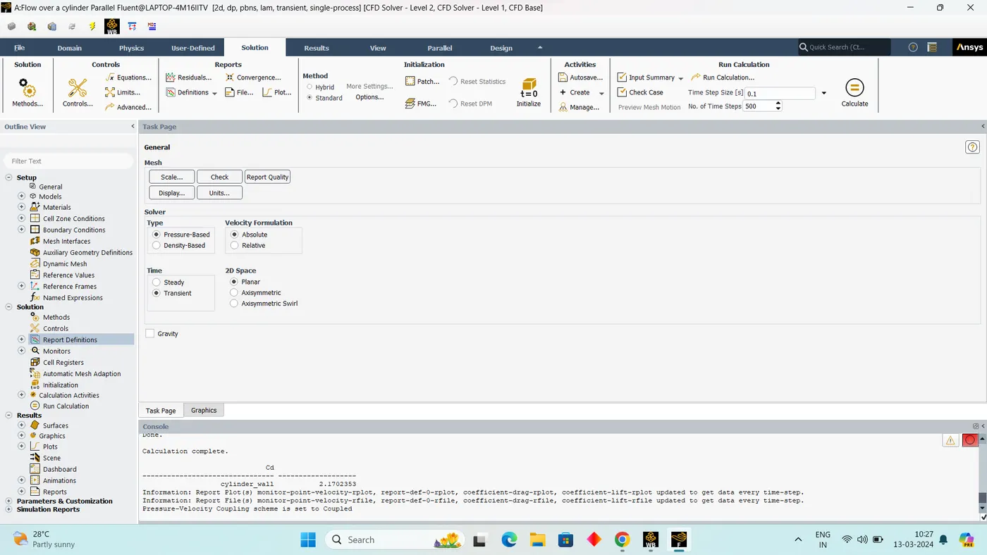
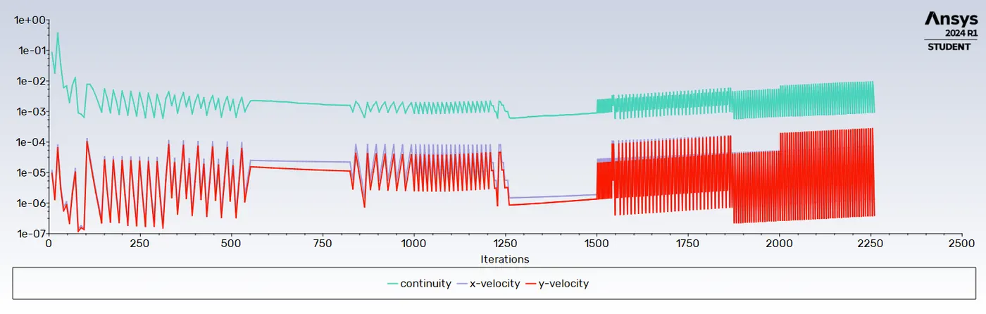
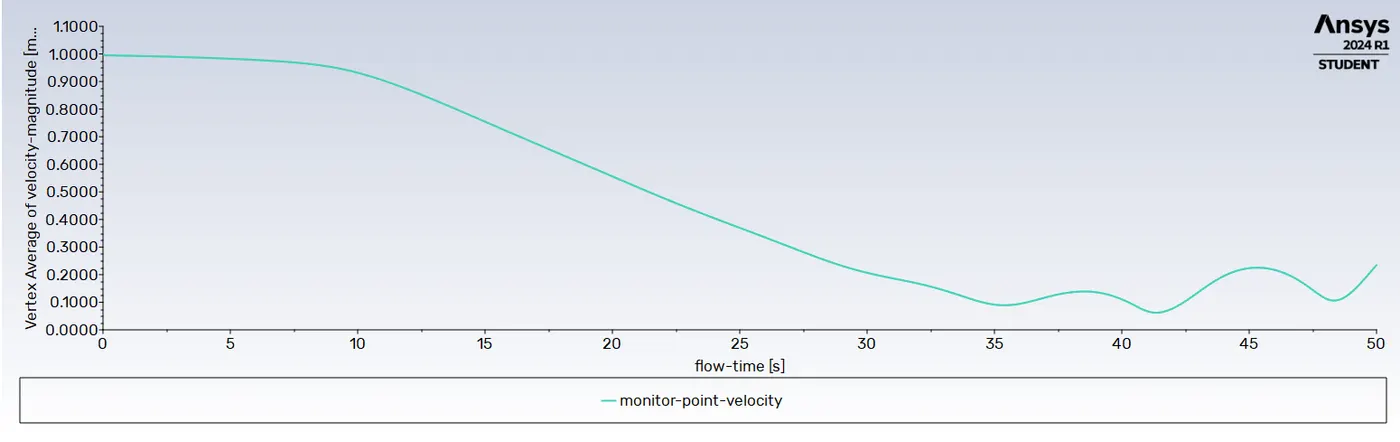
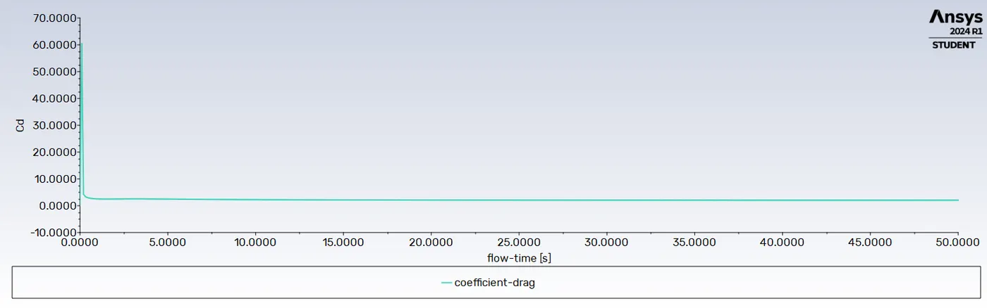
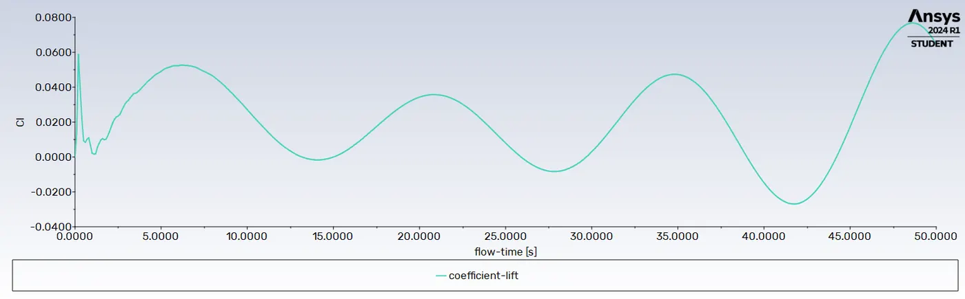
Transient analysis considers changes in the flow variables over time. It models the dynamic behavior of the system.

Time-Dependence:

The governing equations include time derivatives, allowing for the simulation of time-varying conditions.

Convergence:

Convergence is achieved when the solution stabilizes over both space and time.

Applications:

Suitable for scenarios with dynamic events, start-up or shutdown processes, unsteady flows, and interactions with moving objects (e.g., fluid-structure interaction).

Advantages:

Captures time-dependent phenomena and transient events.

Provides a more accurate representation of certain physical processes.

Limitations:

Requires longer computation times and more computational resources.

Convergence criteria become more complex due to the time-dependent nature of the simulation.

 

PART:II

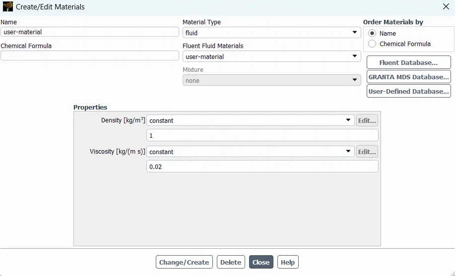
Calculating the velocity for different Reynold's number

`Re = (rho v D) / mu`

Density,`rho`= 1 `(kg)/(m^3)`

Diameter, D = 2 m

Dynamic Viscosity `mu=0.02 (kg)/(ms)`

To find the Velocity V for different Reynold's numbers 

`Re=(1 * v *2)/ 0.02`

`v = 0.010 Re`

CASE	Reynold's Number	Velocity (m/s)
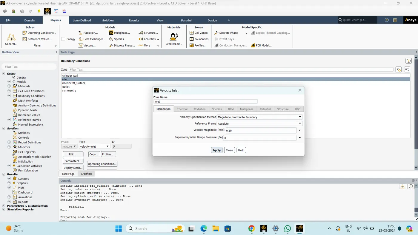
CASE I	10	0.10
CASE II	100	1.0
CASE III	1000	10
CASE IV	10000	100
CASE V	100000	1000

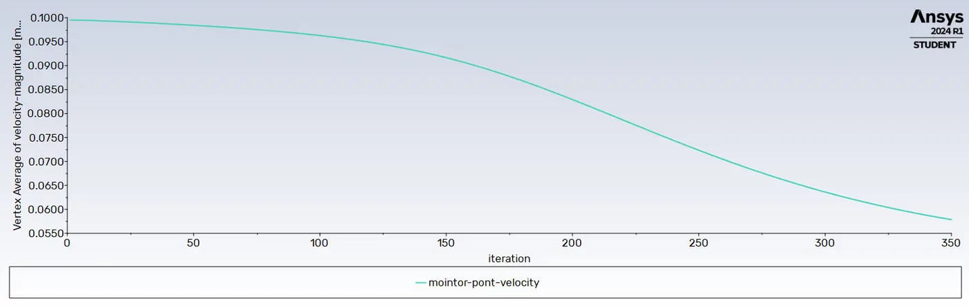
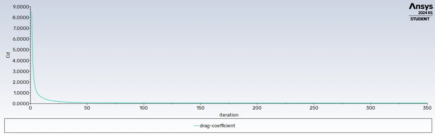
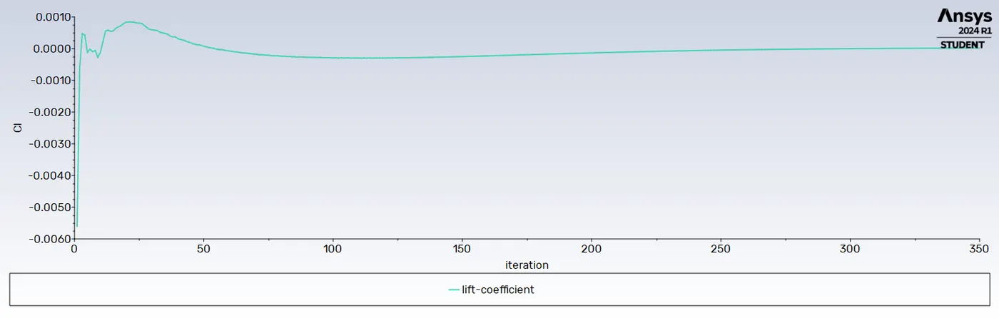
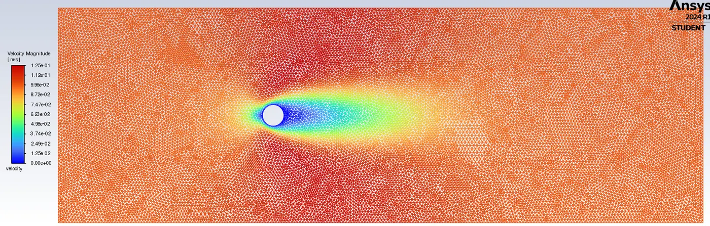
CASE I

Re = 10, Velocity v = 0.1 m/s

VIDEO LINK: https://youtu.be/Jk0edLJ2vrg

 CASE II

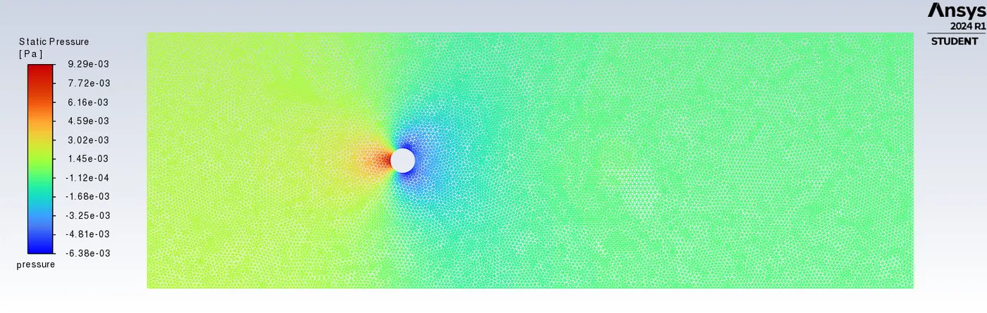
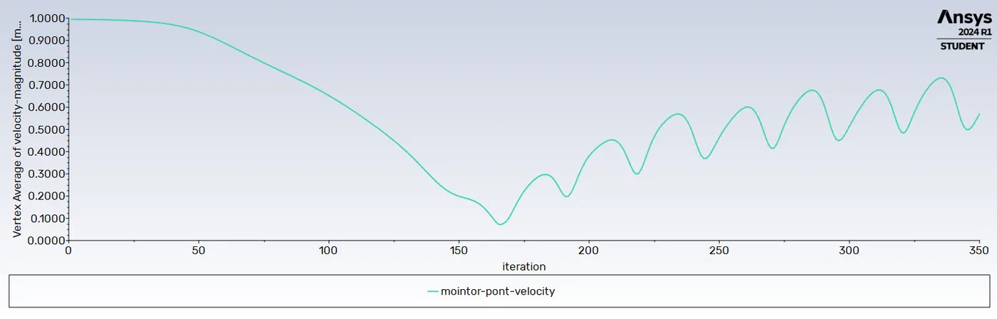
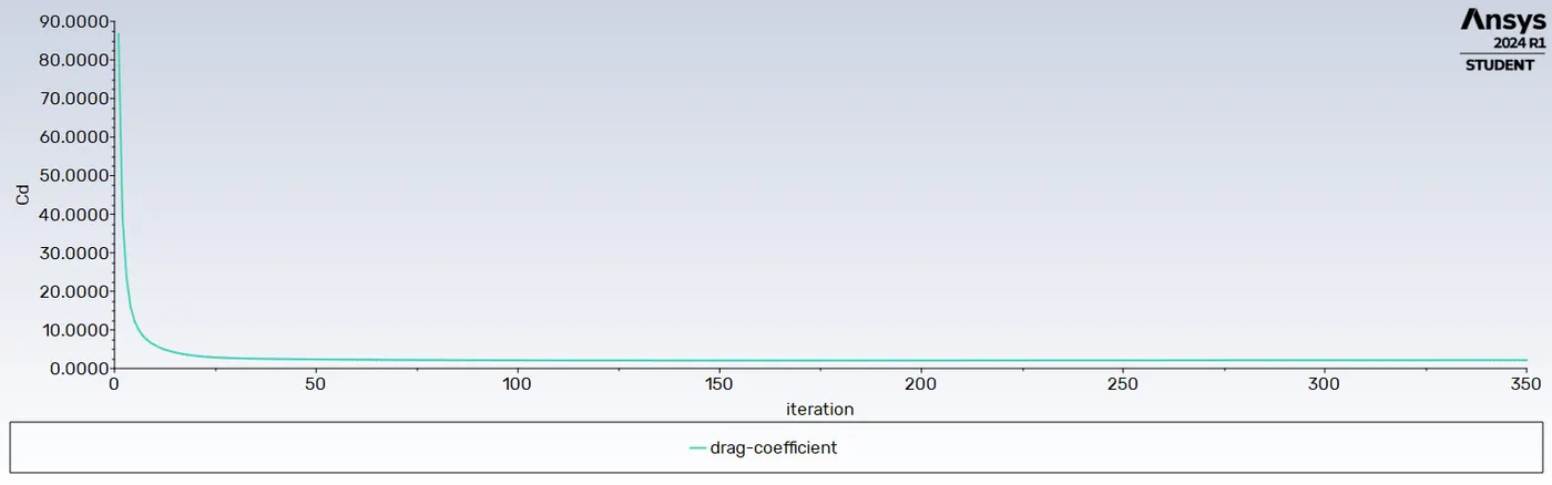
Re - 100, Velocity v - 1 m/s.

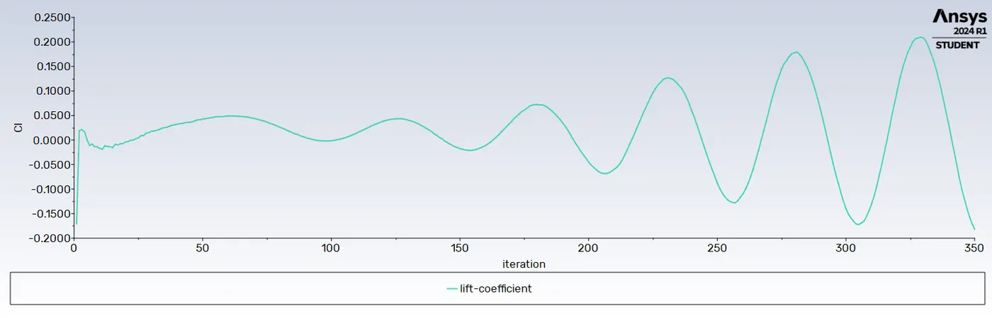
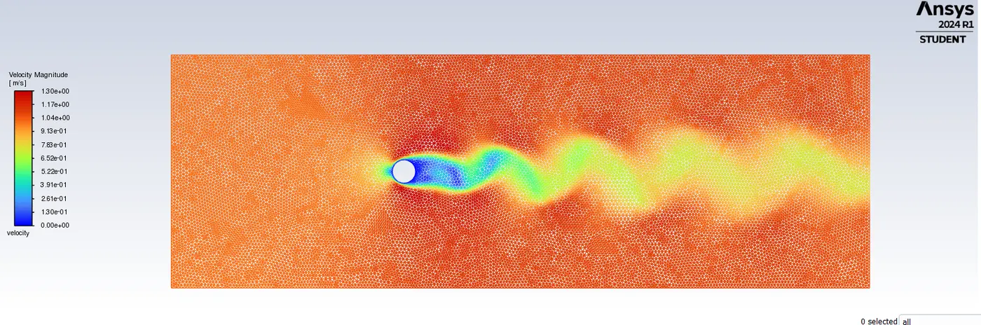
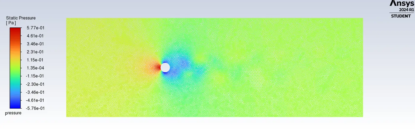
 VIDEO LINK: https://youtu.be/FGQl3Ab8e5A

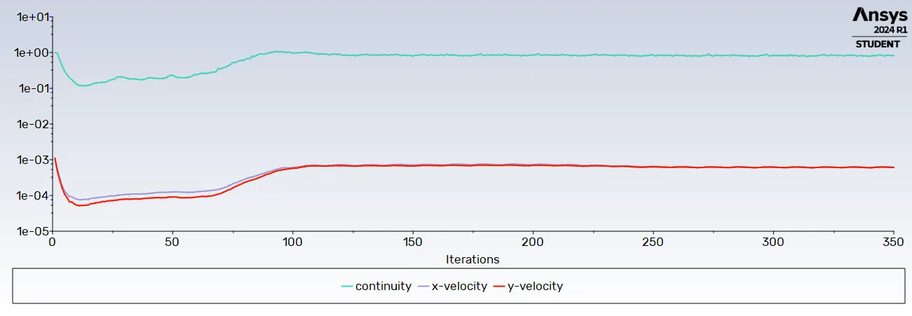
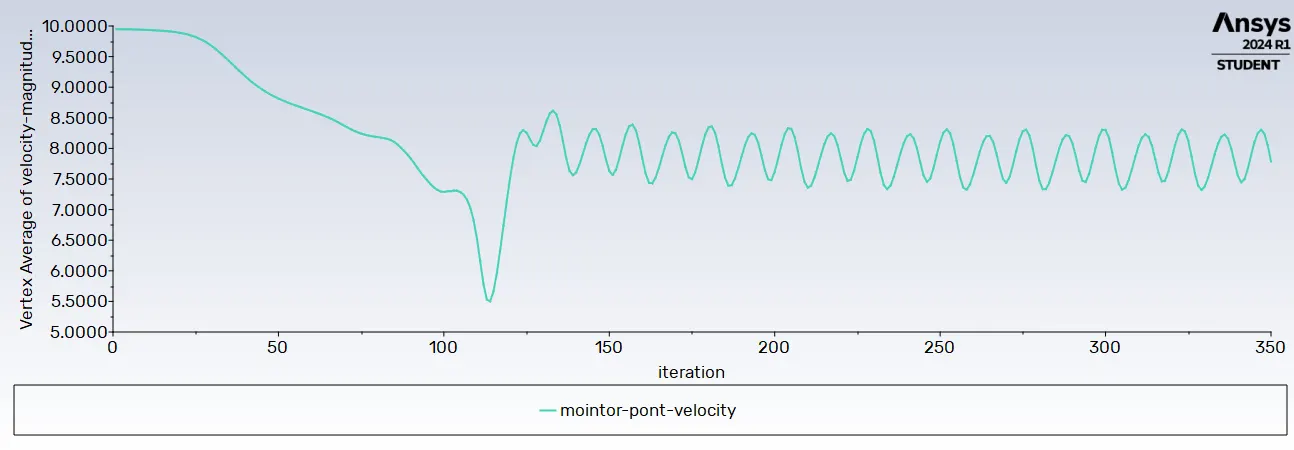
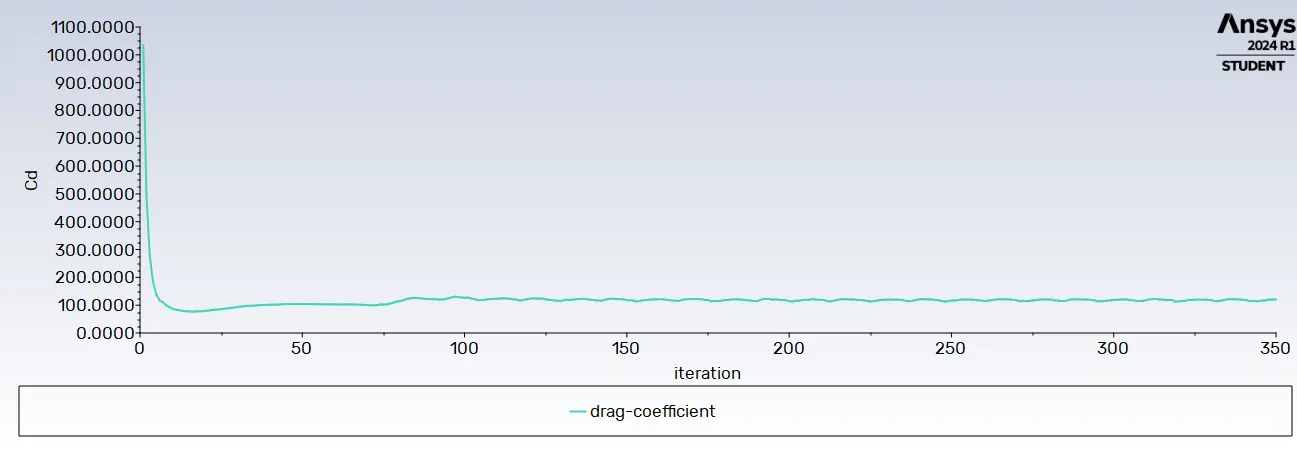
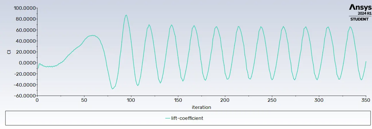
CASE III

Re - 1000, Velocity v - 10 m/s.

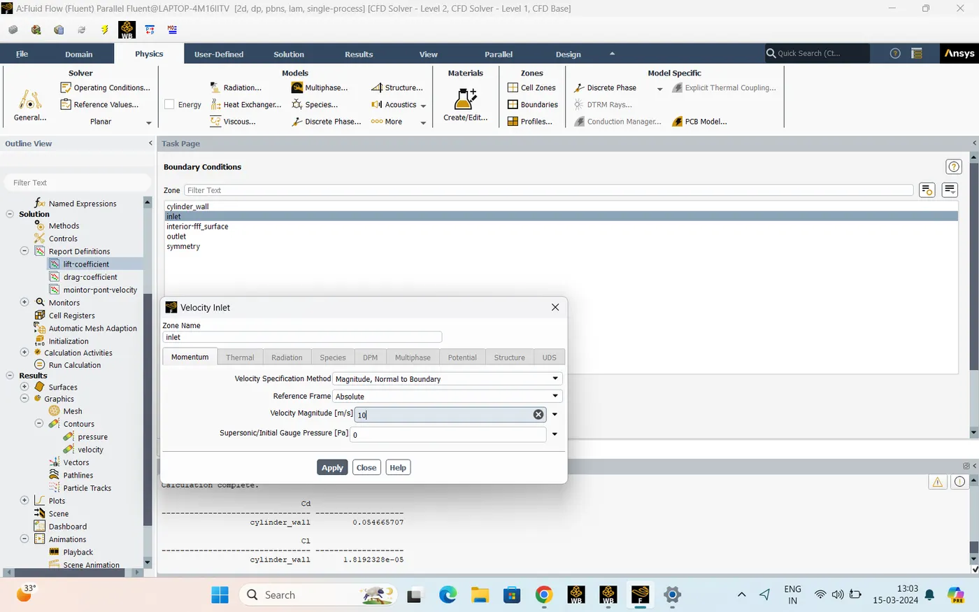
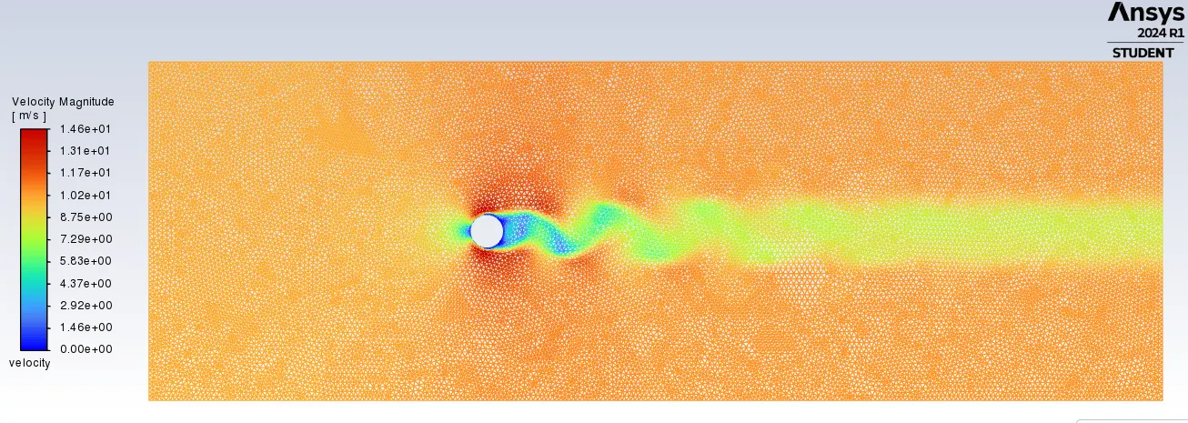
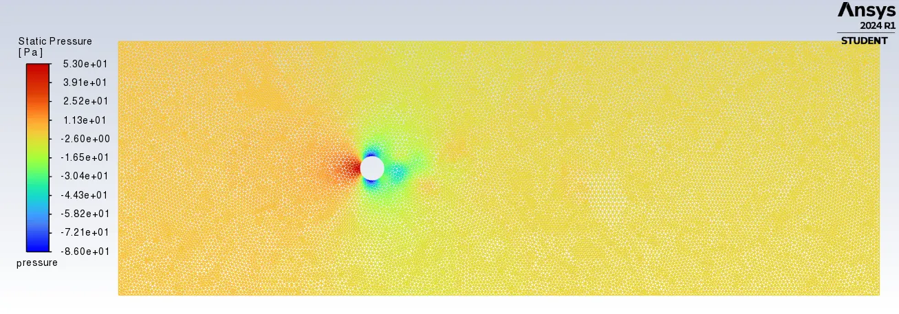
VIDEO LINK: https://youtu.be/nRFDB-gpvbY

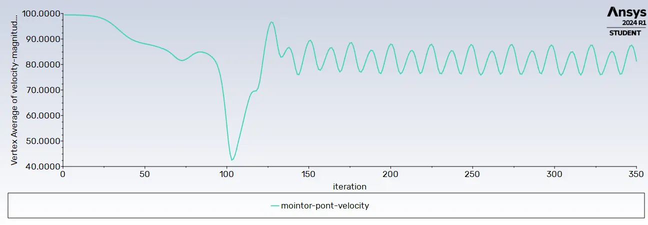
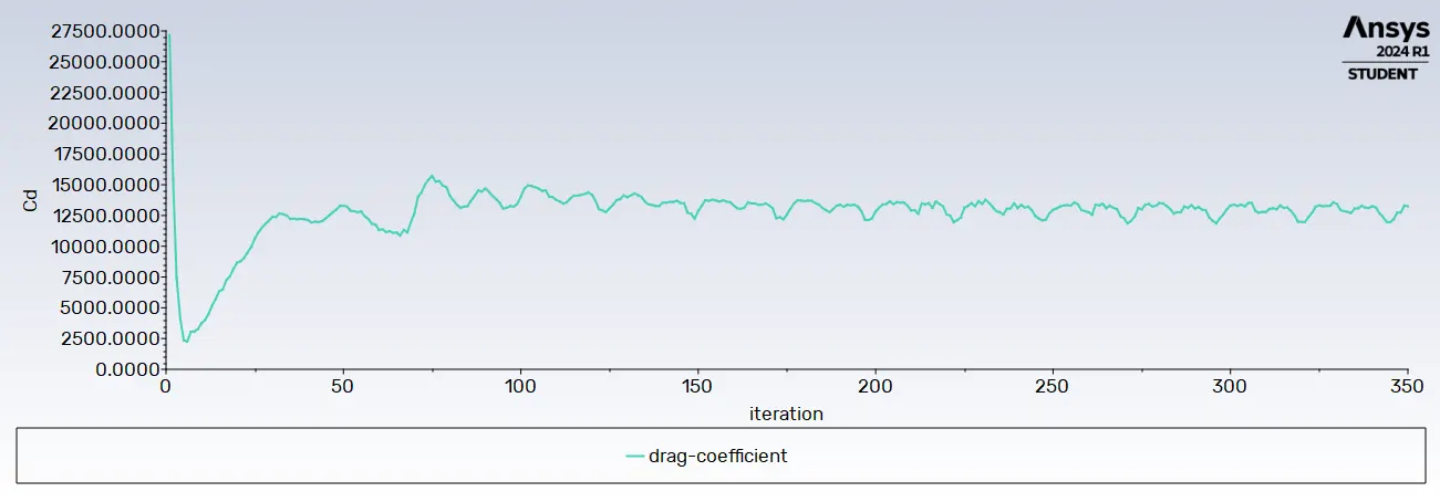
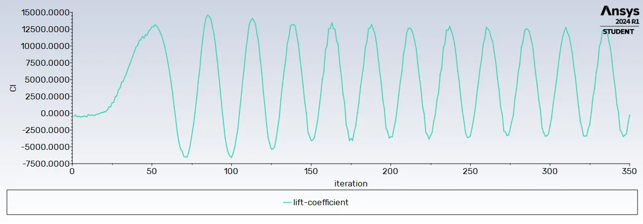
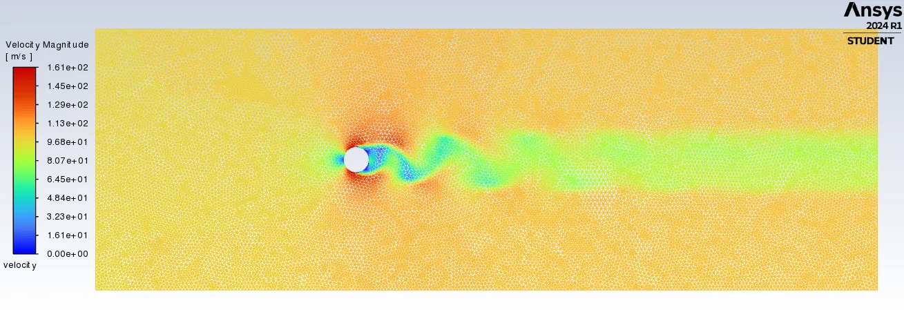
CASE IV

 Re - 10000, Velocity v - 100 m/s.

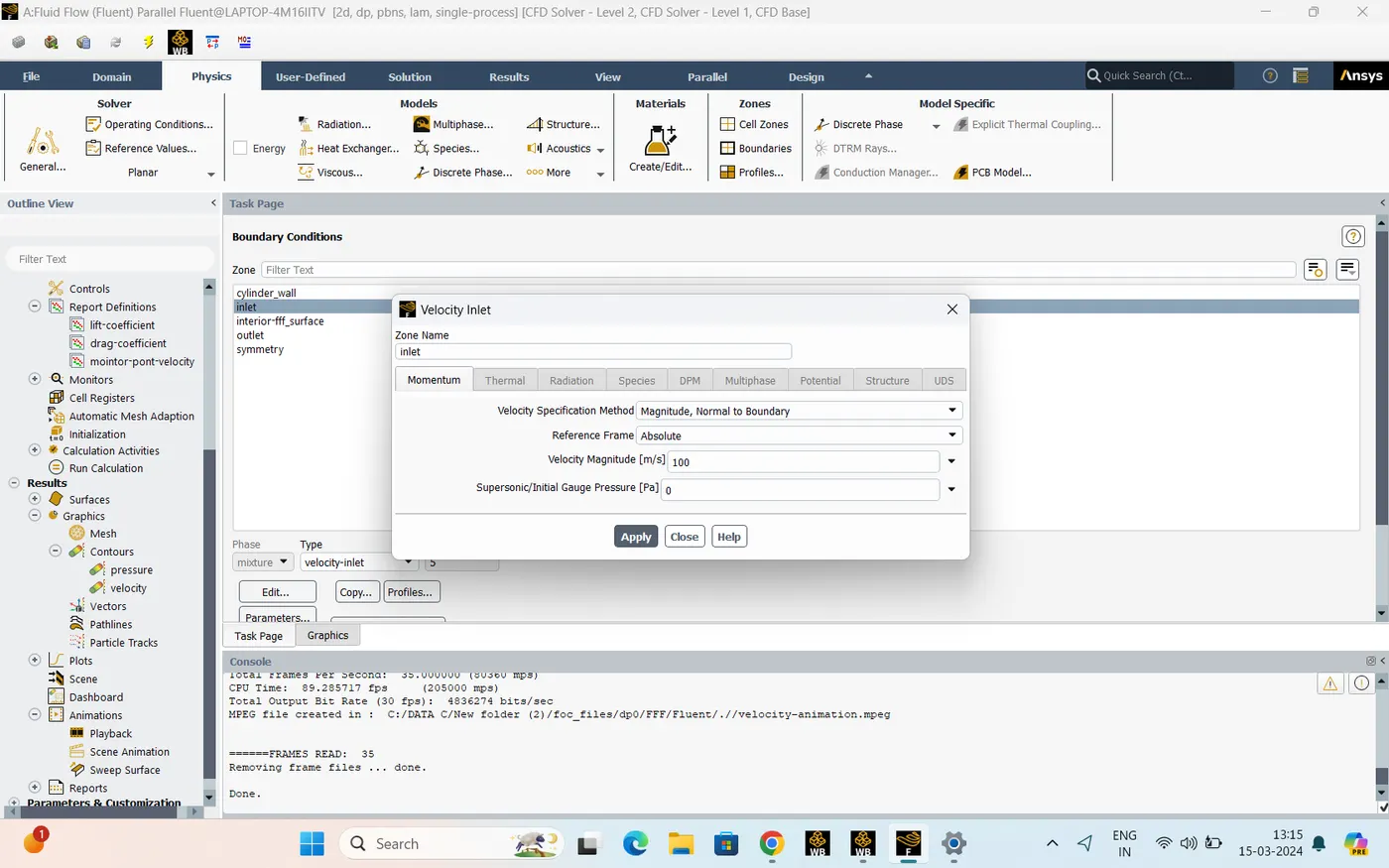
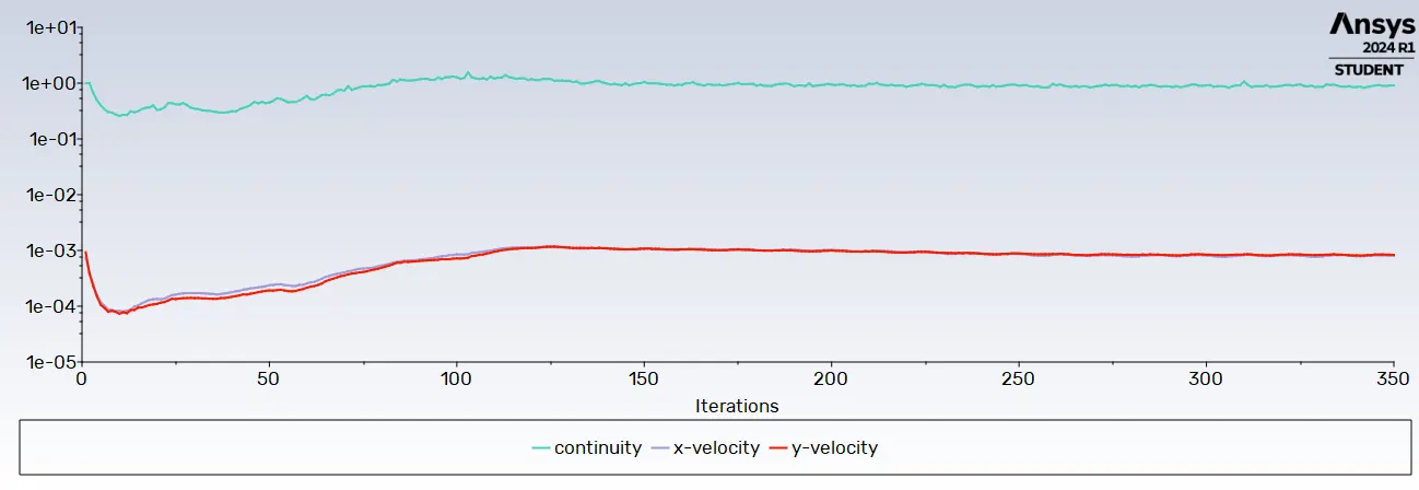
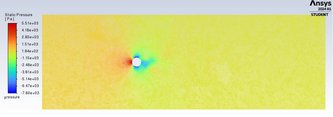
 VIDEO LINK: https://youtu.be/sbEQth8r2KQ

CASE V

 Re - 100000, Velocity v - 1000 m/s.

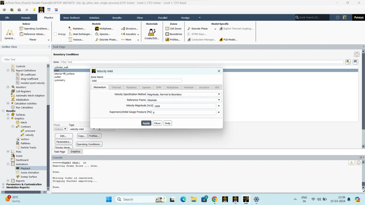
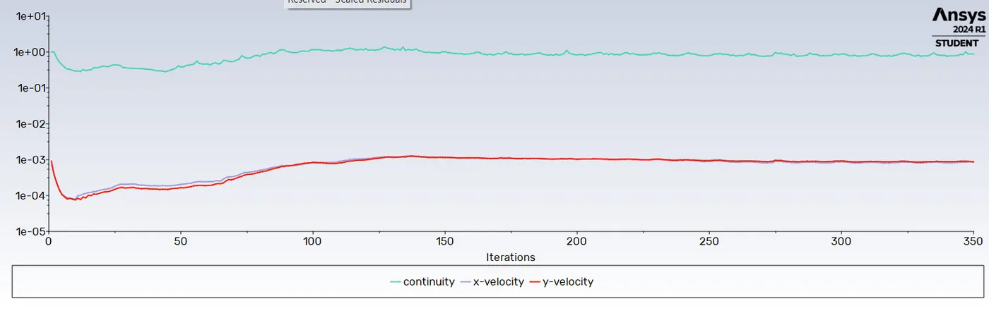
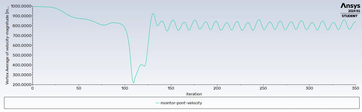
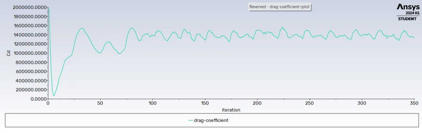
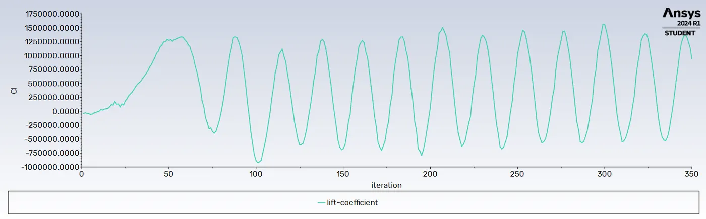
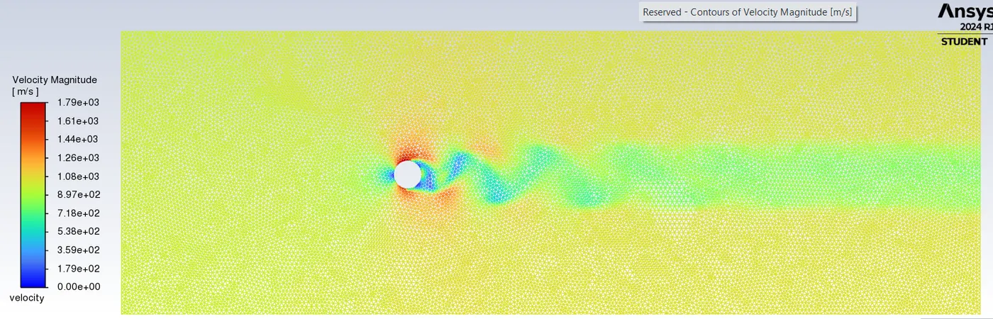
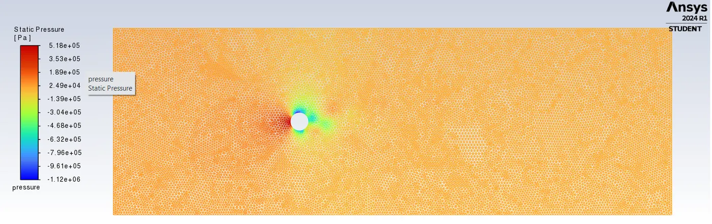VIDEO LINK: https://youtu.be/01EHhLRhYVM

RESULTS:

1. 1. Study of Karman Vortex Street Phenomenon:

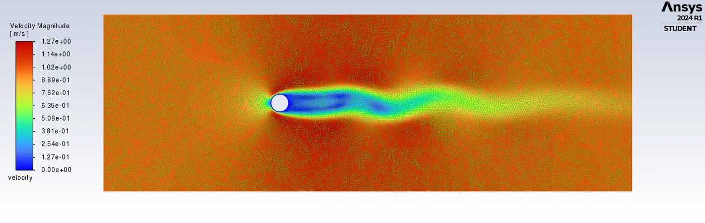
2. This refers to the observation of the alternating pattern of swirling vortices generated when a fluid flows past a bluff body, such as a cylinder. Understanding this phenomenon is crucial in various engineering applications, including aerodynamics and fluid mechanics.

3. 2. Effect of Velocity on Drag:

4. As the velocity of the fluid flow increases, the drag force experienced by the cylinder also increases. In some cases, the turbulent drag may surpass the laminar drag. However, during the transition from laminar to turbulent flow, there exists a range of Reynolds numbers where the turbulent drag is actually lower than the laminar drag. This transitional region is of interest for its unique flow characteristics and potential engineering implications.

5. 3. Vortex Shedding in Steady and Transient Simulations:

6. Vortex shedding, which is the periodic shedding of vortices in the wake of a bluff body, can be observed in both steady-state and transient (time-dependent) simulations. However, it's noted that transient simulations tend to yield better and more realistic results. This is likely because transient simulations capture the time-dependent behavior of the flow more accurately, including the shedding frequency and vortex formation.

7. 4. Strouhal Number Calculation:

8. The Strouhal number (��St) is a dimensionless quantity used to characterize the vortex shedding frequency relative to the flow velocity and characteristic length scale of the bluff body. In transient simulations, the shedding frequency varies with time, necessitating the calculation of the Strouhal number at different time intervals. This parameter is valuable for predicting and analyzing the vortex shedding phenomenon and its impact on drag and flow patterns.

REFERENCES:

1. Li, J. & Chambarel, A. & Donneaud, M. & Martin, R.. (1991). Numerical study of Laminar flow past one and two circular cylinders. Computers & Fluids. 19. 155-170. 10.1016/0045-7930(91)90031-C. 
2. B. N., Rajani & Kandasamy, A. & Majumdar, Sekhar. (2009). Numerical simulation of laminar flow past a circular cylinder. Applied Mathematical Modelling. 33. 1228-1247. 10.1016/j.apm.2008.01.017. 
3. Norberg, C. (1994). An experimental investigation of the flow around a circular cylinder: influence of aspect ratio. Journal of Fluid Mechanics, 258, 287-316.