Week 2 - Flow over a Cylinder.
Introduction:
Frequently, a walker who observes the water running behind bridge pillars can see vortices with opposite signs shed alternatively from either side of the obstacle. These vortices are called " Von Karman Street ". This regular pattern of vortices in the wake is called a Karman vortex street. It creates an oscillating flow at a discrete frequency that is correlated to the Reynolds number of the flow. The periodic nature of the vortex shedding phenomenon can sometimes lead to unwanted structural vibrations, especially when the shedding frequency matches one of the resonant frequencies of the structure. This is a complex phenomenon on which a lot of studies have been made and published, but it can be explained easily with the notion of swirling sheets instabilities. In the fifteenth century, Leonardo da Vinci sketched a row of vortices in the wake of a piling in a stream. In 1878, Strouhal found that the Aeolian tones generated by a wire in the wind were proportional to the wind speed divided by the wire thickness. He noticed that the sound greatly increased when the natural tones of the wire coincided with the Aeolian tones. In 1879, Lord Raleigh found that a violin string in a chimney draft vibrated primarily across the flow, rather than with the flow. The periodicity of the wake of a cylinder was associated with vortex formation by Benard in 1908 and with the formation of a stable street of staggered vortices by von Karman in 1912.
A Kármán vortex street (or a von Kármán vortex street) is a repeating pattern of swirling vortices, which is caused by a process known as vortex shedding. It is responsible for the unsteady separation of flow of a fluid flow around the blunt bodies. Von Karman vortices form almost everywhere where the fluid flow is disturbed by an obstruction.
When a fluid particle reaches Infront of the obstruction the pressure drops on the account of velocity and becomes stagnation pressure. From the leading edge of the cylinder boundary layer, development can be observed. Due to the non-slip condition, the shear layer velocity will be different for different layers and hence the shear layer will be rolling into the near wake where they fold on each other and coalesce into discrete swirling vortices. And such a regular pattern of vortices called a " Von Karman vortices”. The phenomenon arises under certain flow conditions, expressed commonly by the dimensionless Reynolds number.
`Re_L=(VL)/ν`
`Re_L=(ρVL)/μ`
where,
V= the free stream flow velocity (m/s)
L= characteristic length parameter of the body or channel (m)
`ρ=` the reference fluid density `((kg)/m^3)`
`nu=` kinematic viscosity (=dynamic viscosity/density=`mu/rho`) `(m^2/s)`
The image below shows a von Karman vortex street develops behind a cylinder moving through a fluid.
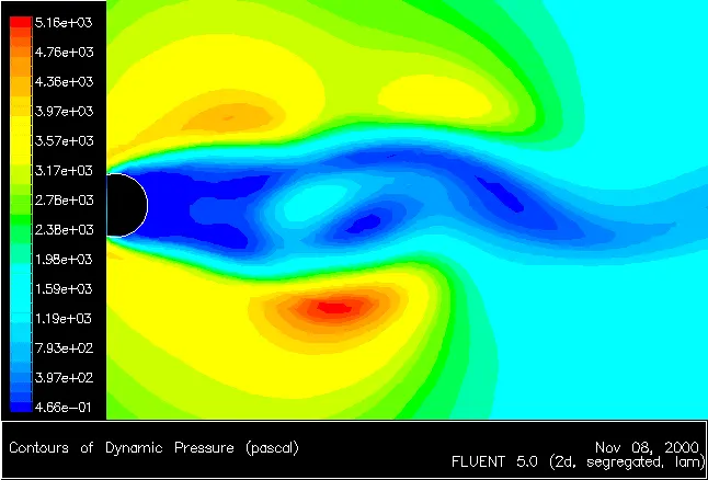
When a single vortex is shed, an asymmetrical flow pattern forms around the body and changes the pressure distribution. This means that the alternate shedding of vortices can create periodic lateral (sideways) forces on the body in question, causing it to vibrate. If the vortex shedding frequency is similar to the natural frequency of a body or structure, it causes resonance. It is this forced vibration that, at the correct frequency, causes suspended telephone or power lines to "swing" and the antenna on a car to vibrate more strongly at certain speeds.
In dimensional analysis, the Strouhal number is a dimensionless number describing oscillating flow mechanisms. The Strouhal number is an integral part of the fundamentals of fluid mechanics.
Strouhal number, `St=(f*l)/U`
where, `f=`frequency; `L=`characteristic length (diameter of the cylinder in our case); and `U=`flow velocity.
According to Newton's second law, time rate change of the linear momentum is equal to the sum of all external forces acting on a system. Therefore, an integration of the linear momentum inside a control volume surrounding the circular cylinder can provide information of the aerodynamic forces (lift and drag) acting on the cylinder. There are alternative upward and downward flows in the wake as the result of vortex shedding. Consequently, there must be also an oscillatory up and downforce acting periodically on the cylinder. This periodic forcing exerting on the cylinder body is responsible for the vortex-induced vibrations as described earlier.
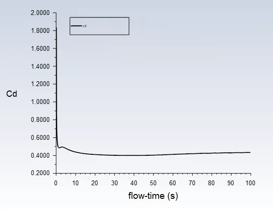
Finally, defining the drag coefficient `(C_d)` and the lift coefficient `(C_L)` as:
`C_d=(2*F_d)/(ρ*V^2*A)` and `C_L=(2*F_L)/(ρ*V^2*A)`
where,
`F_d=`Drag Force (N)
`F_L`=Lift Force (N)
`rho=` density of the fluid `((kg)/m^3)`
`V=`Flow velocity`(m/s)`
`A=`Cross sectional area `(m^2)`
PRE-PROCESSING:
Geometry:
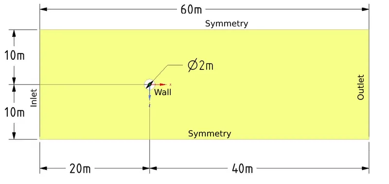
SpaceClaim is used for geometry creation. Geometry dimensions are shown below.
Meshing:
We use ANSYS inbuilt Meshing tool for the meshing.
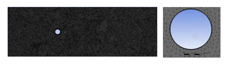
All triangular method is inserted for meshing. For the sake of representing the circular wall almost as a circle instead of a polygon edge sizing is used and a total number of 36 divisions are provided. To get a body-fitted mesh inflation layers are inserted. a total of 6 inflation layers have been included with a 5 mm first layer thickness. The growth rate is specified as 1.2. The element size has been chosen as 0.25m and we’re getting a number of nodes=41534 and a number of elements=40642. Named selections are created for inlet, outlet, wall and the symmetry planes. The snapshot of the meshed geometry is given below.
For the simulation, a user-defined material has been considered with a density of 1 `(kg)/m^3` and dynamic viscosity of 0.02 `(kg)/(m.s)`
Since the flow is considered to be incompressible the pressure-based solver is used along with absolute velocity formulation.
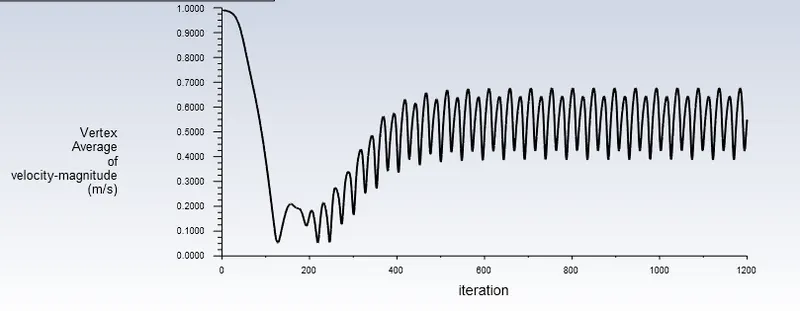
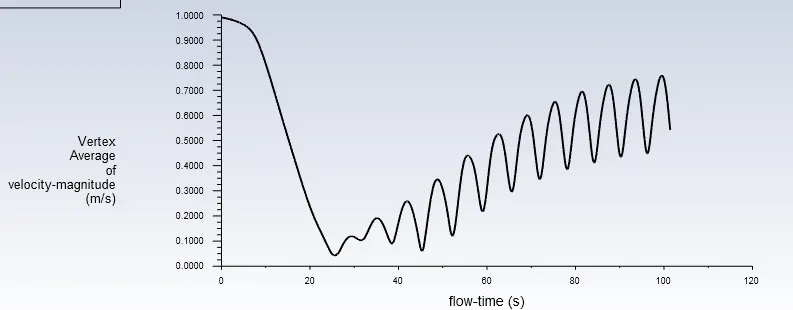
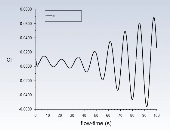
A monitor point at a distance of 4D (8m) to the right side of the cylinder has been created in order to capture the vortex-shedding behind the cylinder. The Coordinates of the point was (8, 0). After creating the monitor-point a vertex average surface report with velocity as the parameter has been generated defined on it. Another two force reports have been defined for capturing coefficient of lift and drag with the wall of the cylinder as the reference surface. under the reference value section calculate from the inlet option is chosen. And hybrid initialization is used to set up the initial condition for the entire flow field.
To visualize the flow field pressure and velocity contours have to be defined from the post-processing section for respective parameters.
In order to create the solution animation From the ‘Activities’ tab, ‘solution animation’ has been selected and frames were defined to record for after every 10 iterations velocity was selected as the parameter to be visualized.
For steady-state solver simulation was run for 1200 iterations and for transient-state solver ran up to 1000 timesteps with a step size of 0.1 seconds.
PART-I:
a) Simulation with the steady-state solver, Dynamic viscosity = 0.02 `(kg)/(m.s)` and Re = 100
A steady-state solver with the laminar viscous model has been used to simulate the problem. The SIMPLE scheme with the least square cell-based system for gradients is used. Pressure and Momentum interpolation schemes were chosen as second-order and second-order upwind.
at the Inlet velocity inlet boundary condition has been used with inlet velocity equals to 1m/s. At the outlet pressure-outlet condition is used with gauge pressure equals to zero. At the walls, the no-slip condition is given and the bottom and top boundaries were treated with symmetry boundary condition.
The results are given below.
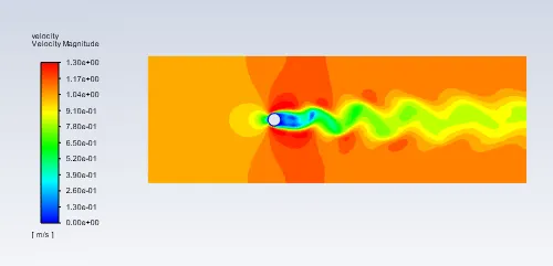
Velocity Contour:
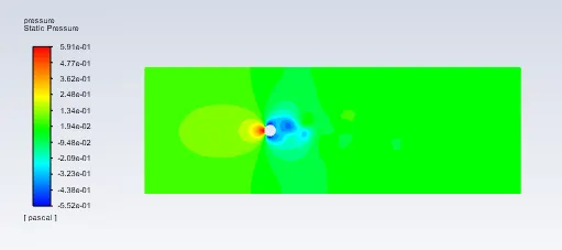
Pressure Contour:
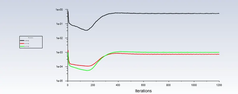
Residual Plot
Vertex average velocity plot
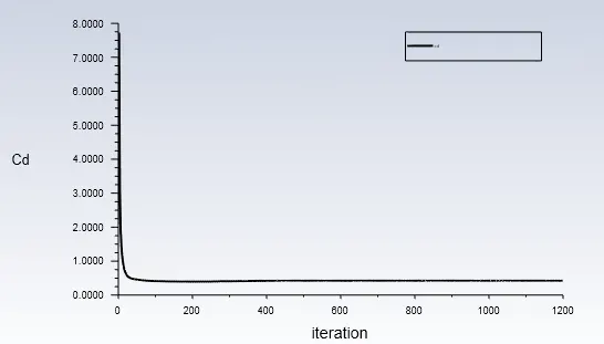
Coefficient of Drag plot:
Coefficient of Lift plot:
Solution Animation
b) Simulation with the transient solver, Dynamic viscosity = 0.02 `(kg)/(m.s)` and Re = 100
A transient solver with the laminar viscous model has been used to simulate the problem. The SIMPLE scheme with the least square cell-based system for gradients is used. Pressure and Momentum interpolation schemes were chosen as second-order and second-order upwind.
at the Inlet velocity inlet boundary condition has been used with inlet velocity equals to 1m/s. At the outlet pressure-outlet condition is used with gauge pressure equals to zero. At the walls, the no-slip condition is given and the bottom and top boundaries were treated with symmetry boundary condition.
The results are given below.
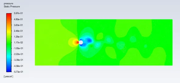
pressure contour
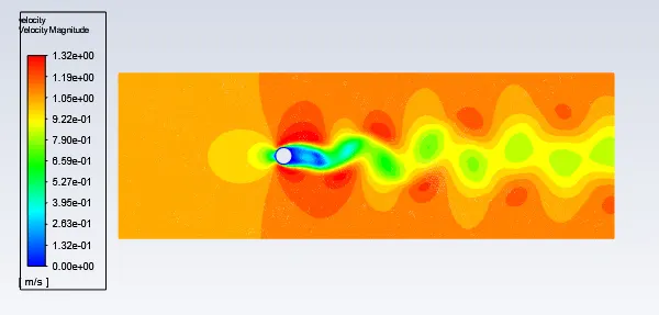
Velocity Contour:
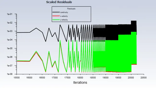
Residual Plot
Vertex average velocity plot
Coefficient of Drag plot:
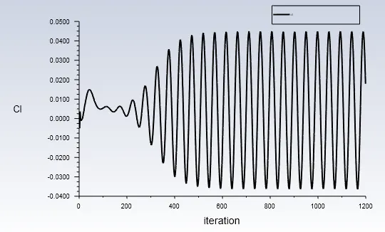
Coefficient of Lift plot:
Solution Animation
Strouhal Number Calculation.
We know that Strouhal Number
`St = (fD)/U`
where f is the vortex shedding frequency, D is the diameter of the cylinder, and U is the free-stream velocity. If we found out the vortex shedding frequency strouhal number can be calculated. For that, a MATLAB program has been made which requires a 3 column matrix (A), which is the output file of the coefficient of lift from Ansys fluent.
clear all
close  all
clc
A=[];
for i = 1: length(A)
  time(i) = A(i,3);
  cl(i)= A(i,2);
end
 plot(time,cl)
 pks = findpeaks(cl);

 for k = 1:length(time)
     if cl(k) == pks(length(pks)-1)
         t1 = time (k);
     elseif cl(k) == pks(length(pks))
         t2 = time(k);
     end
 end
 f = 1/(t2-t1)
 D =2;
 U=1;
 St = (f*D)/U
The obtained strouhal number was 0.1681
CONCLUSION:
The transient simulation is more realistic since it takes account of the parameter time in the governing equation. For the transient process like vortex shedding, it's better to use transient simulation to get realistic output.
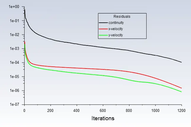
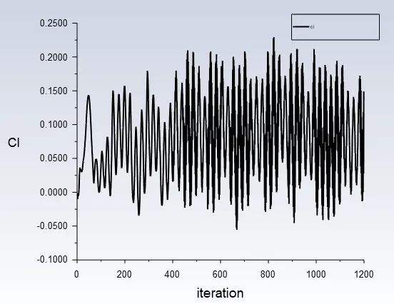
From the 500th iteration onwards for the steady-state simulation, we can observe a periodic oscillatory for the residuals, vortex averaged velocity and coefficient of lift and a constant value for the coefficient of drag which implies that the solution is converged.
It's meaningless to monitoring the residuals to say that the simulation has reached a steady state. It gives the time-wise development of the phenomenon.
PART-II:
Re 10
A steady-state solver with the laminar viscous model has been used to simulate the problem. The SIMPLE scheme with the least square cell-based system for gradients is used. Pressure and Momentum interpolation schemes were chosen as second-order and second-order upwind.
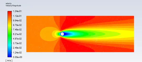
at the Inlet velocity inlet boundary condition has been used with inlet velocity equals to 0.1m/s. At the outlet pressure-outlet condition is used with gauge pressure equals to zero. At the walls, the no-slip condition is given and the bottom and top boundaries were treated with symmetry boundary condition.
The results are given below.
pressure contour
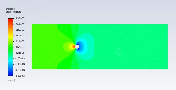
Velocity Contour:
residual plot
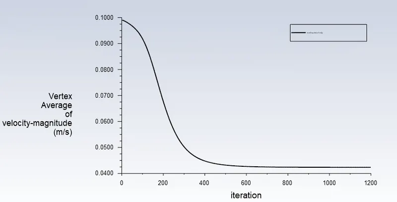
Plot for Vertex average of Velocity:
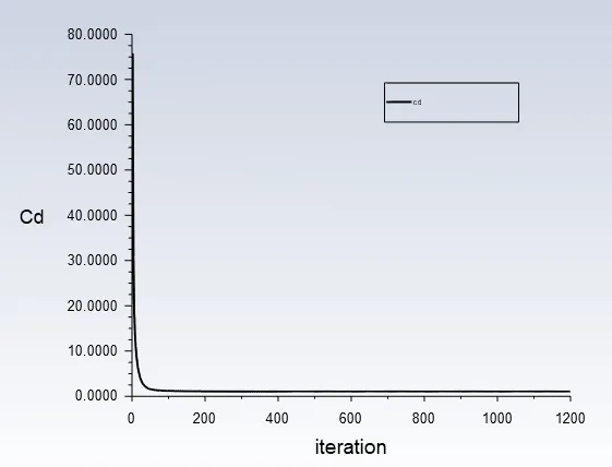
Coefficient of Drag plot:
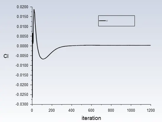
Coefficient of Lift plot:
Solution Animation
Re 100
A steady-state solver with the laminar viscous model has been used to simulate the problem. The SIMPLE scheme with the least square cell-based system for gradients is used. Pressure and Momentum interpolation schemes were chosen as second-order and second-order upwind.
at the Inlet velocity inlet boundary condition has been used with inlet velocity equals to 1m/s. At the outlet pressure-outlet condition is used with gauge pressure equals to zero. At the walls, the no-slip condition is given and the bottom and top boundaries were treated with symmetry boundary condition.
The results are given below.
Velocity Contour:
pressure contour :
residual plot
Plot for Vertex average of Velocity:
Coefficient of Drag plot:
Coefficient of Lift plot:
Solution Animation
Re 1000
A steady-state solver with the SST K-Omega viscous model has been used to simulate the problem. The SIMPLE scheme with the least square cell-based system for gradients is used. Pressure and Momentum interpolation schemes were chosen as second-order and second-order upwind.
at the Inlet velocity inlet boundary condition has been used with inlet velocity equals to 10m/s. At the outlet pressure-outlet condition is used with gauge pressure equals to zero. At the walls, the no-slip condition is given and the bottom and top boundaries were treated with symmetry boundary condition.
The results are given below.
pressure contour
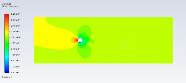
Velocity Contour:
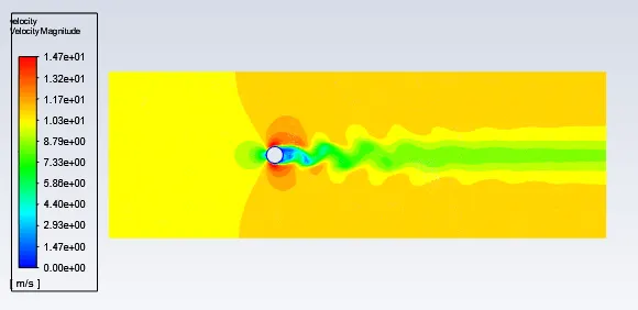
residual plot
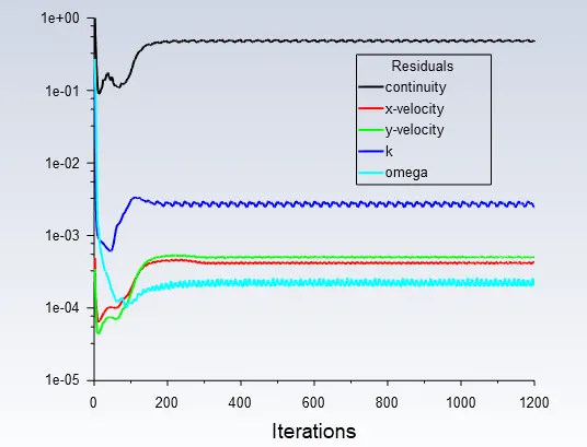
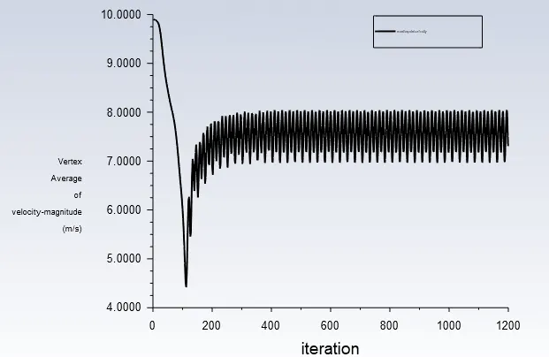
Plot for Vertex average of Velocity:
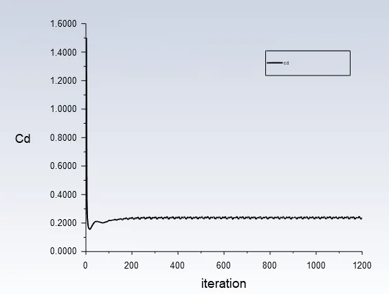
Coefficient of Drag plot:
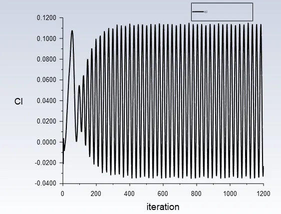
Coefficient of Lift plot:
Solution Animation
Re 10000
A steady-state solver with the SST K-Omega viscous model has been used to simulate the problem. The SIMPLE scheme with the least square cell-based system for gradients is used. Pressure and Momentum interpolation schemes were chosen as second-order and second-order upwind.
at the Inlet velocity inlet boundary condition has been used with inlet velocity equals to 100 m/s. At the outlet pressure-outlet condition is used with gauge pressure equals to zero. At the walls, the no-slip condition is given and the bottom and top boundaries were treated with symmetry boundary condition.
The results are given below.
pressure contour :
Velocity Contour:
residual plot
Plot for Vertex average of Velocity:
Coefficient of Drag plot:
Coefficient of Lift plot:
Solution Animation
Re 100000
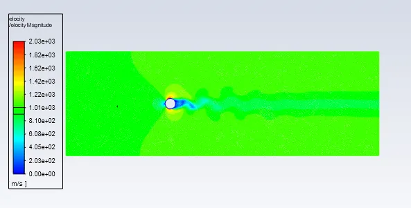
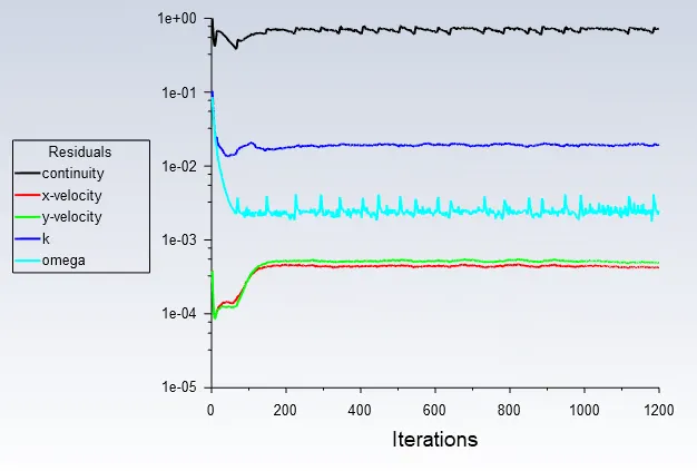
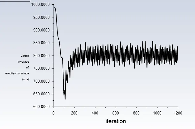
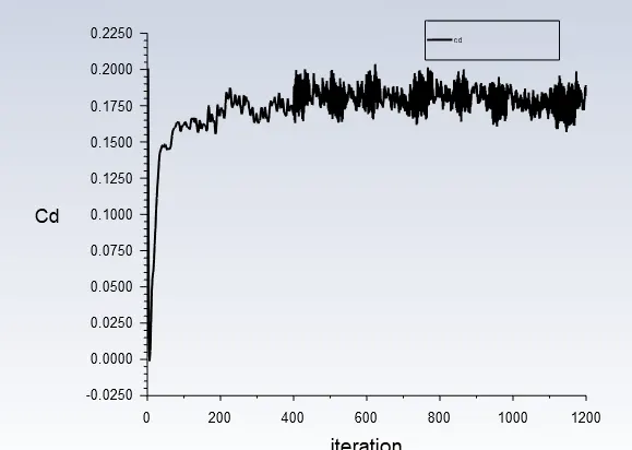
A steady-state solver with the SST K-Omega viscous model has been used to simulate the problem. The SIMPLE scheme with the least square cell-based system for gradients is used. Pressure and Momentum interpolation schemes were chosen as second-order and second-order upwind.
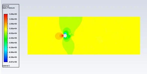
at the Inlet velocity inlet boundary condition has been used with inlet velocity equals to 1000 m/s. At the outlet pressure-outlet condition is used with gauge pressure equals to zero. At the walls, the no-slip condition is given and the bottom and top boundaries were treated with symmetry boundary condition.
The results are given below.
pressure contour
Velocity Contour:
residual plot
Plot for Vertex average of Velocity:
Coefficient of Drag plot:
Coefficient of Lift plot:
Solution Animation
The
| Reynolds number | Inlet Velocity (m/s) | coefficient of drag | coefficient of lift |
| 10 | 0.1 | 1.0588 | 0.00029934 |
| 100 | 1 | 0.4260 | 0.0056086 |
| 1000 | 10 | 0.2371 | 0.041297 |
| 10000 | 100 | 0.2465 | 0.1081 |
| 100000 | 1000 | 0.1799 | 0.088114 |
CONCLUSION:
As the Reynold number is increased the vortices are shed alternately from the upper and lower surface of the cylinder at a definite frequency which is a function of Reynolds number. When the Reynolds number becomes greater than 1000 the oscillations were found to be increasing. As the Reynolds number increases, inertial forces dominate over viscous forces. The coefficient of drag (Cd) is found to be decreasing and the oscillatory nature of the coefficient of lift is observed. The mean value of Vertex average of Velocity and coefficient of lift is found to be increasing with Reynolds number.
From the table, we can notice that as we increase the Reynolds number, our Drag coefficient is decreasing whereas the Lift coefficient increasing. When we compare these results with the findings of Rajani et al. [2], we found that our results agreed reasonably well.
But contrastingly the drag coefficient for Re = 10000 case should be less than that of Re = 1000 case. And the value of the Lift coefficient should be less than the values obtained from the Re=100000 simulation.
It can be can observed that along with an increase in the Reynolds number, the flow becomes more and more unsymmetrical. Increasing velocity eventually brings the turbulent drag up to and even higher than the laminar drag value.
References:
https://en.wikipedia.org/wiki/Kármán_vortex_street
B.N. Rajani, S. Majumdar, A. Kandasamy, Numerical simulation of laminar flow past a circular cylinder, Applied Mathematical Modelling 33 (2009) 1228–1247