Week 2 - Flow over a Cylinder.
AIM: 2-D flow simulation for circular cylinder to investigate the vortex shedding phenomena interms of the Strouhal number and to evaluate the variation of Coefficient of Lift and Drag with increasing Reynolds number.
Introduction: Flow over a circular cyllinder is basically flow over a bluff body which doesn't allow the boundary layers to combine. Over the decades, numerous efforts are put in to investigate this geometry because of the occurance of vortex shedding phenomena. When fluid passes through the cylinder, flow gets saperated due to adverse pressure gradient. The seperation results into two contra-rotating vortices/eddies, when the saperated boundary layers interact vortices are shed. Vortices are formed around any oject of any shape, its occurance is possible for viscous flows only. Depending upon the reynolds number the vortex shedding can be periodic or abrupt. The pattern is not only mesmarizing to watch but it significant consequences on Aerodynamics of object.
Theorey:
1. Flow Seperation due to Adverse Pressure Gradient
Gradient of pressure = Force due to pressure = -∇.P= Pressure force acting in direction of decreasing pressure magnitude, is one of the most important flow variable which dictates the behaviour of flow.
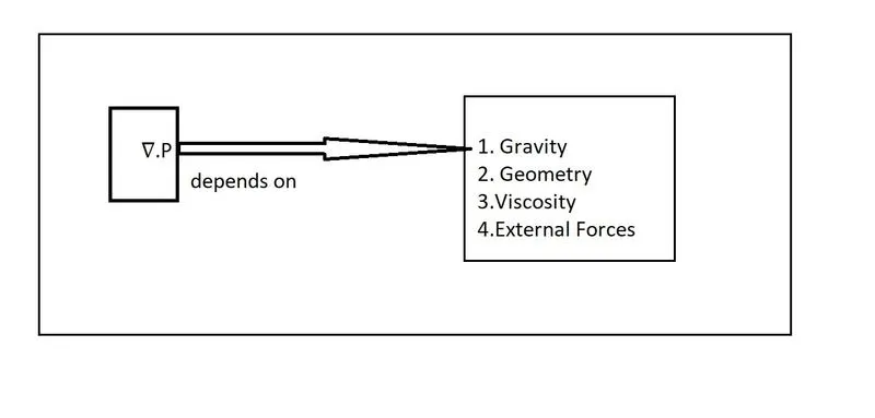
Variation of Gradient of pressure due to geometry leads to flow saperation and formation of Vortices
 [1]
[1]
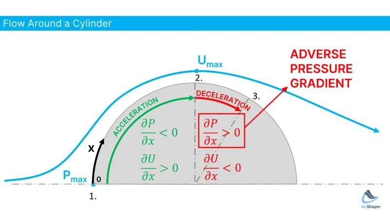
Due to geometry there is a favourable pressure gradient between point 1 and 2. Thus flow is accelerated, pressure decreases and velocity increases. Then again due to curvature of the object the velocity starts to decrease and pressure starts to increase. According to bernaulis theorem the velocity must decrease, this leads to a favourable pressure gradient in the direction normal to surface and leads to boundary layer thickning which is also called the displacement effect. Inside this region pressure increases and stops the fluid point 3. Here fluid has seperated due to adverse pressure gradient as it is not following the curvature of the object. At the point of seperation, the negative pressure gradient reverses the flow and vortices are formed.
Flow past circular cylinder
A cylinder also offers the similar geometry of a bluff object which will cause flow seperation and formation of what is called the Foppl Vortices. It is the interaction of the seperated layers whcih causes vortex shedding. At a particular range of Reynolds number, the vortex shedding occurs periodically and thus at a constant freaquency.
Thus continious vortex shedding can have consquences to the flow mainly interms of drag and lift.
Drag: The resistence offered to the relative motion in between an object and a fluid.
Types of Drag:
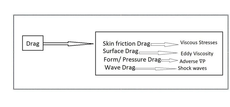
1. Skin friction drag: Due to shear stresses in the boundary layer, can be regared as drag due to viscosity of fluid. Fd,f
2. Surface Drag: Due to Turbulene or the momentum tranfer from eddy viscosity, thus it is the turbulent boundary layer drag.
3. Form Drag: Or pressure drag is the drag that results from Adverse Pressure Gradient. Fd,p
4. Wave Drag: Drag due to Schock waves.
Criteria for vortex shedding
. Interaction between two shear layers having opposite signs is essential for vortices to get cut, become free and cause vortex shedding.
. If simultaneous vortices are forming they will only stretch
. For vortex shedding to take place, one of the seperated layers needs to be ahead of the other.
. The combination of free shedded vortex and the free stream flow, will produce lift which fluctuates between a positive and negative value.
 [2]
[2]
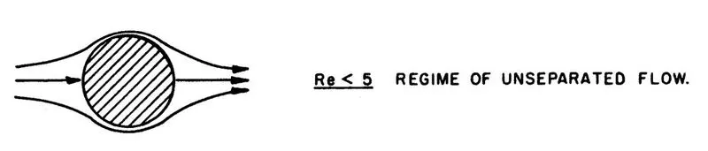
If Re <5 (or in some ther references for Re< 0.3 [ 3] ) the flow behaviour is similar to potential flow there is no vortex formation. Drag is dominated by skin friction drag

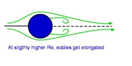
From 2<Re<30, flow seperation occurs and two contra-rotating vortices are formed. Now Pressure drag start dominating
 [3]
[3]
As Re goes over 30 elongation of vortices takes place.
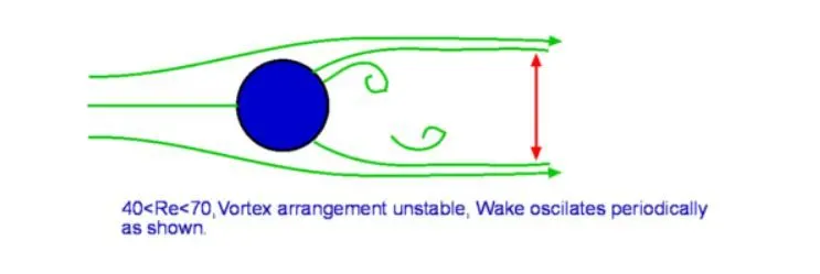
Until now there was only one component of the hydrodynamic force which was Drag, now due to wake oscillation, Lift force starts emerging.
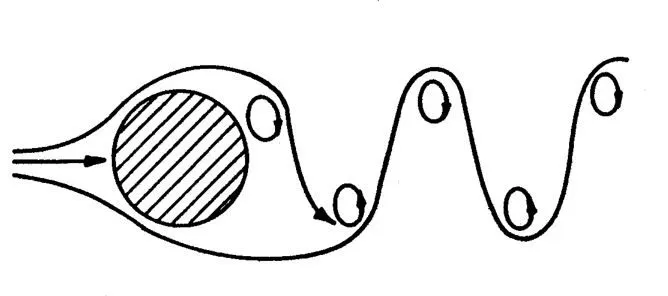
90<Re<150
Pressure Drag = 90% of Total Drag
At around Re=90, one of the seperated layers has proceeded the other, this way both interact down the wake and vortices start shedding, upto Re=150, the vortex shedding occurs periodically and is measured with the strouhal number.
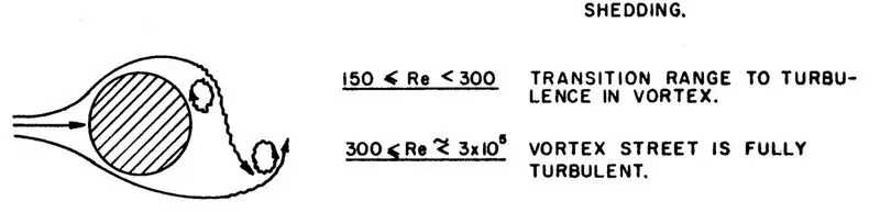
Upto Re=300000, the vortex street is fully turbulent
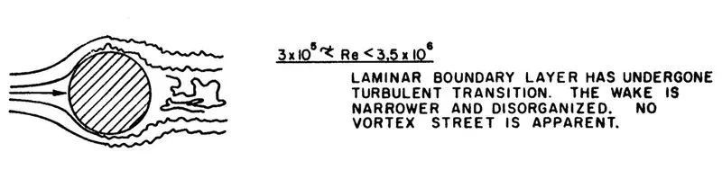
Then as Reynolds number is increased transition to turbulance occurs prior to seperation, as turbulent flow has greater momentum it delays the saperation and wake gets norrower, this leads to what is called Drag crises and reduces the drag coefficient to a minimum of 0.3.
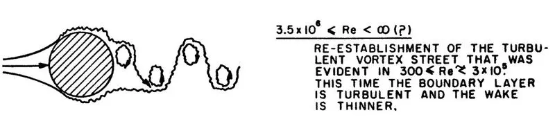
As reynolds number surpasses 3.5 million, the vortex street re-appears and further increases the drag.
Practical significance of Vortex shedding.
The centre of vortes is an area of low pressure thus presence of many vortices like a vortex street represents a region of low pressure, if somehow these vortices appear on the upper part of an airfoil, it will provide additional lift, if it appeared in the lower portion will generate downforce and if appeared in the wake it will incerase Pressure drag and can lead to stall.
Delta Wing Airfoil.
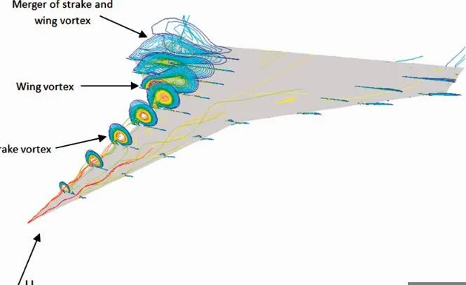
A delta wing based aircraft is common in defence industries such as the Eurofighter Typhoon, Dessault Rafael and HAL Tejas. Their selection for a delta wing airfoil comes from the fact that it can sustain climb at a higher angle of attack without stalling. For a convential airfolil stall angle is around 15 deg and for a Delta it is around 35deg. This is because, at higher angles of attatck vortices are formed on the top which are the regions of low pressure, this induces additional lift on the airfoil and it can climb at higher angles of inclination without stalling.
Solving and Modelling Approach.
Pre-processing
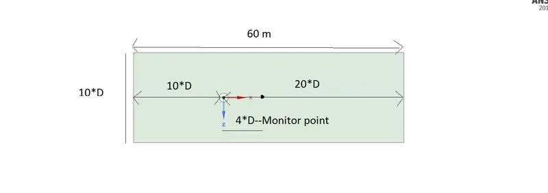
First we draw our 2-D computational domain in ANSYS SPACECLAIM
Meshing
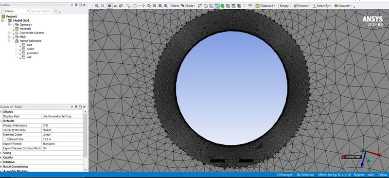
We will use a trangular mesh considering the curvature, but to capture the boundary layers we will employ a body-fitted mesh utilising the inflation layers.
Element size=0.25m
Number of divisions on surface=720
Number of Inflation layers=48
Solver
We will use ANSYS FLUENT for the simulatuion
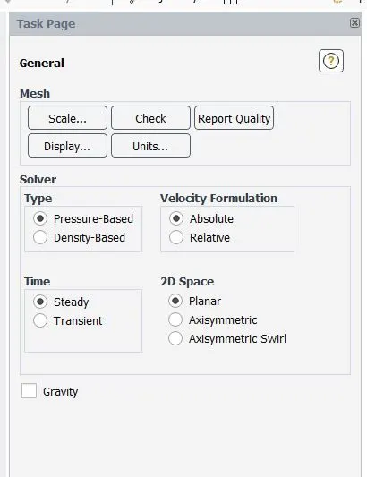
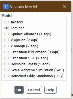
Using Fluent data-base of material we create our own user material so we can vary the reynolds number
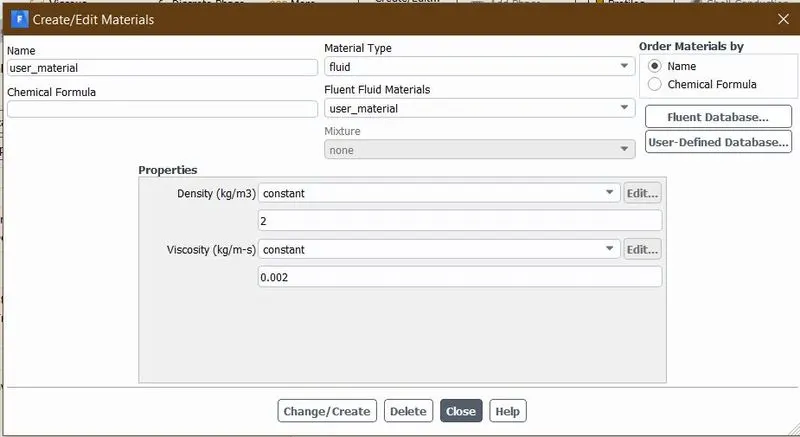
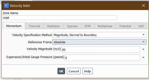
Now we specify the boundars conditions
Inlet
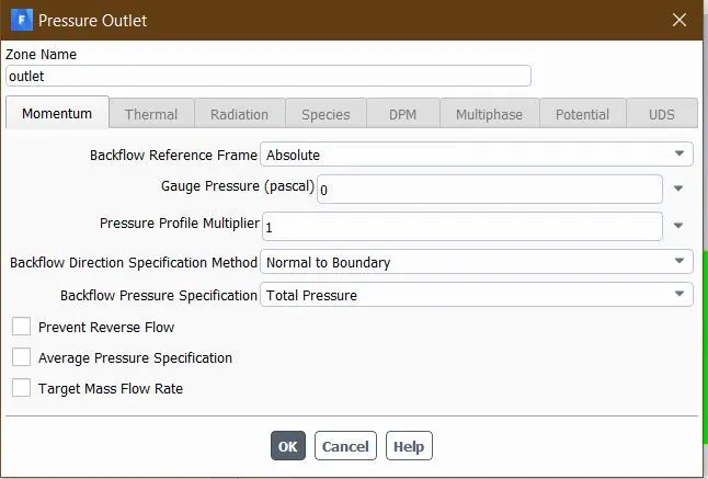
Outlet
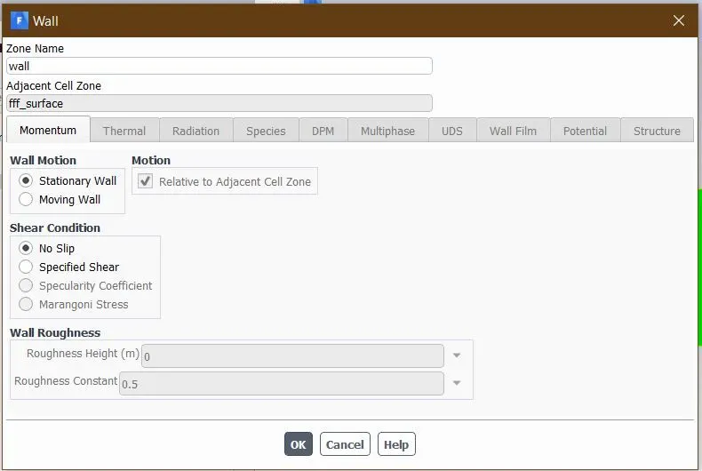
Wall
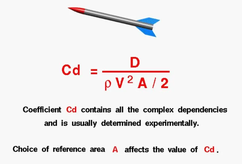
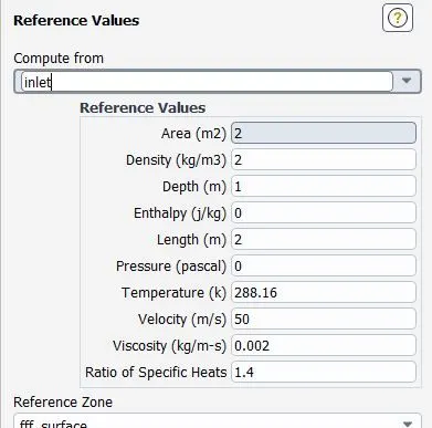
Setting up the Reference Values (critical for Cd and Cl)
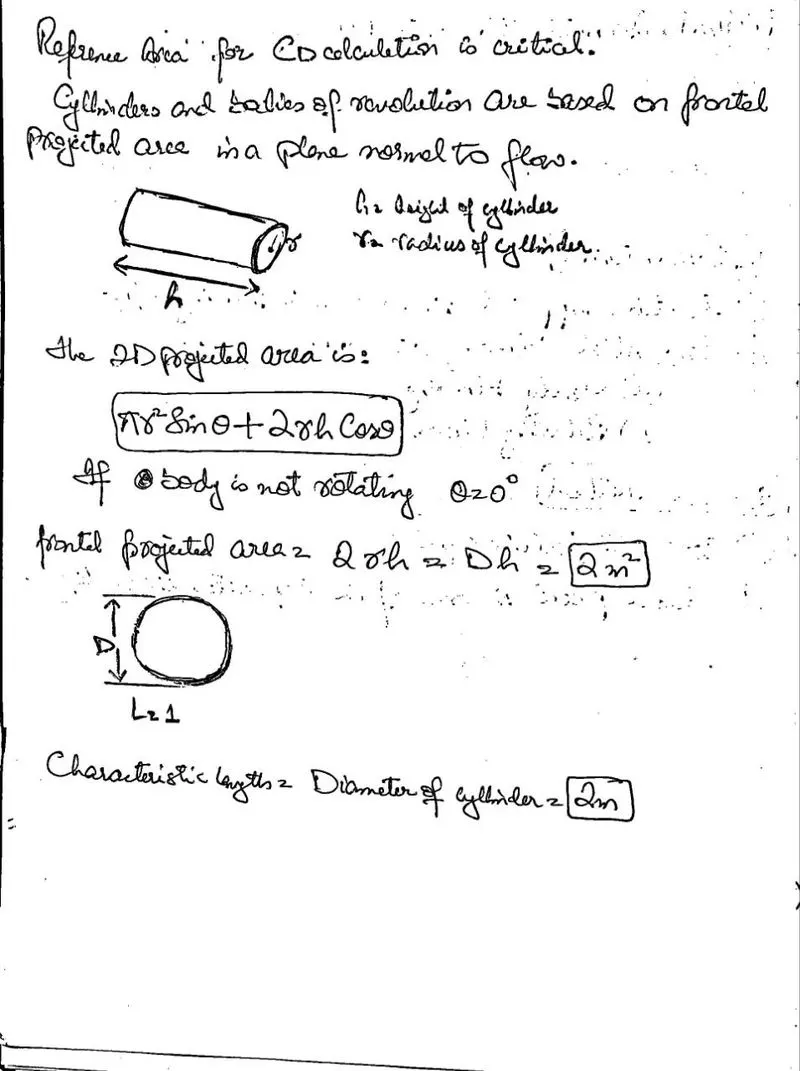 [4 and 5]
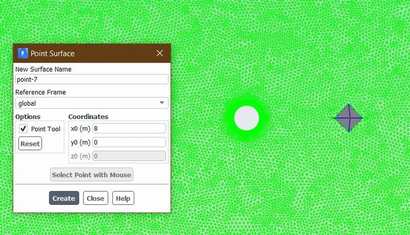
Monitor point to measure velocity fluctuation
Adding Surface Reports
Drag Coefficient
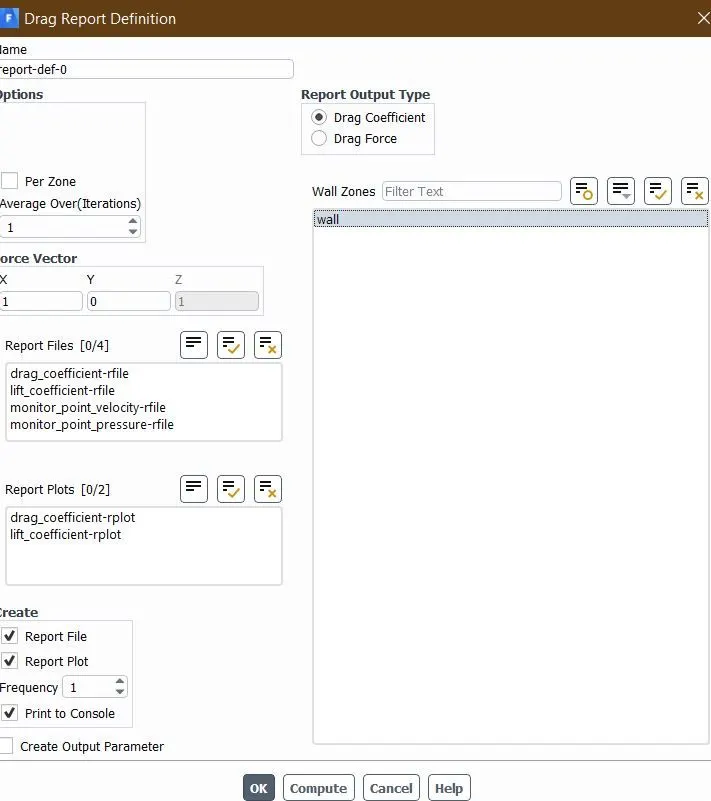
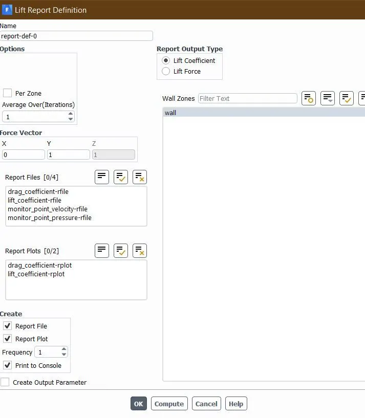
Lift Coefficient
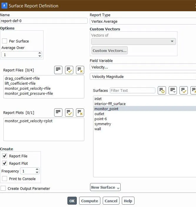
Vortex Average of Velocity at monitor point
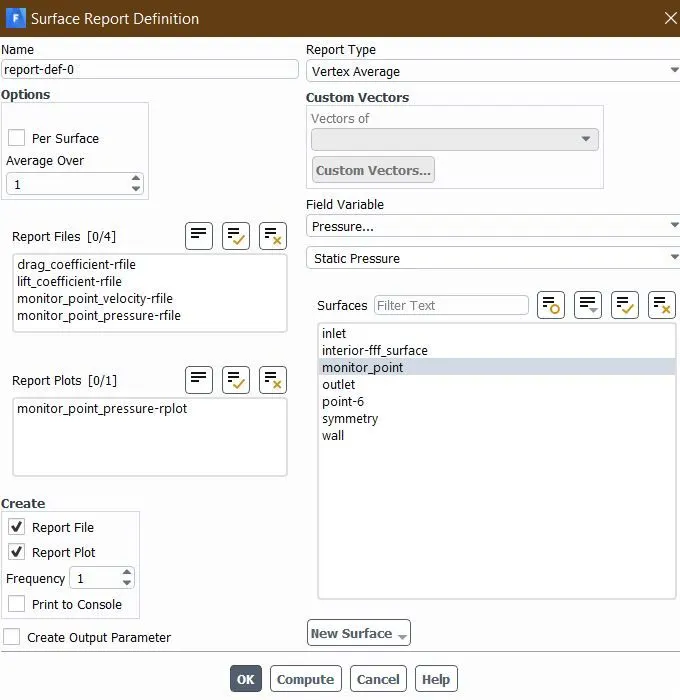
Vortex average of Pressure
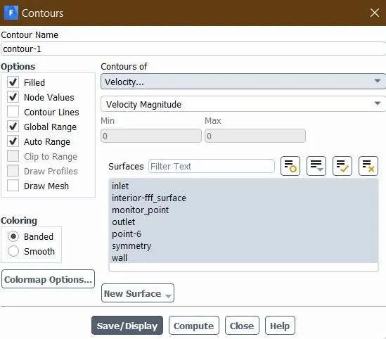
Contour of Velocity
After running the hybrid initialization we can create contours of velocity and pressure
Contour of Pressure
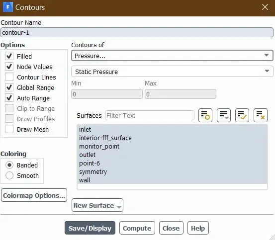
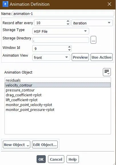
Velocity contour Animation
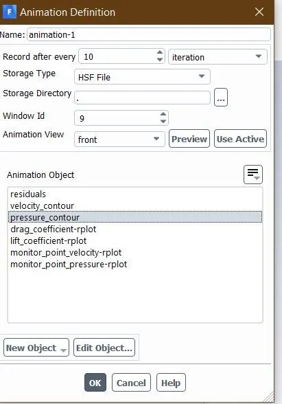
Pressure contour animation
Now we can run the calculation using steady or transient approach
1. Steady flow over Circular Cylinder at Reynolds number 100
Setting Up the Reynolds Number
Re,d=ρ*U*d/µ
Re,d=100
density=1 kg/m^3
d=2m
µ=0.02 kg/ms
U=1m/s
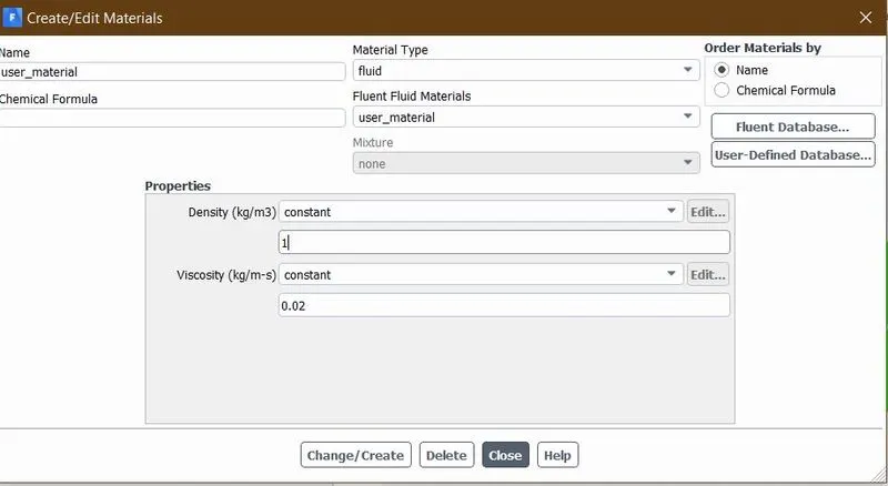
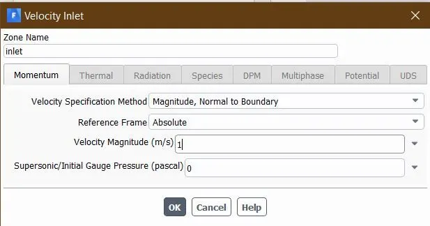
Following our solver setting we run our calculations
1.Scaled Residuals
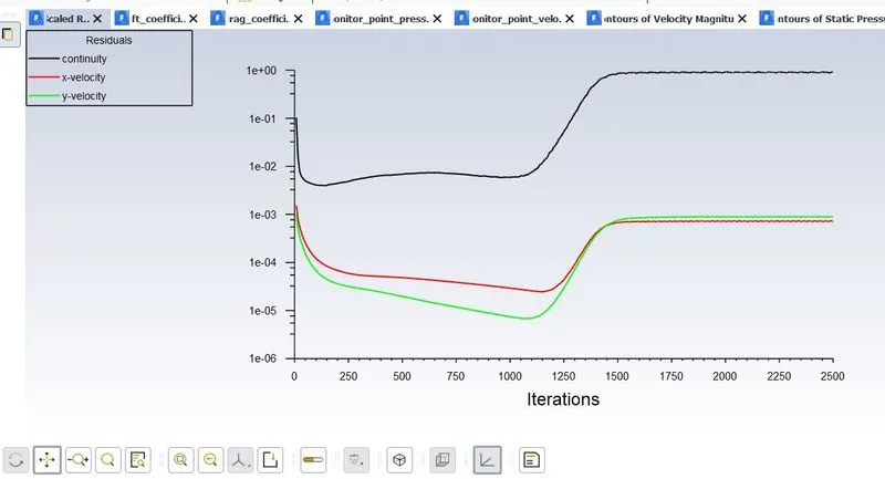
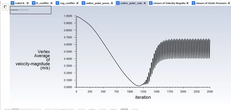
2. Vertex Average of Velocity
3.Vertex Average of Pressure
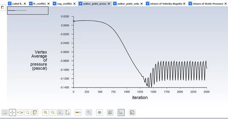
4.Drag Cofficient
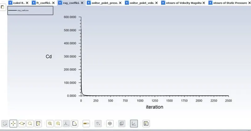
5. Lift Coefficient
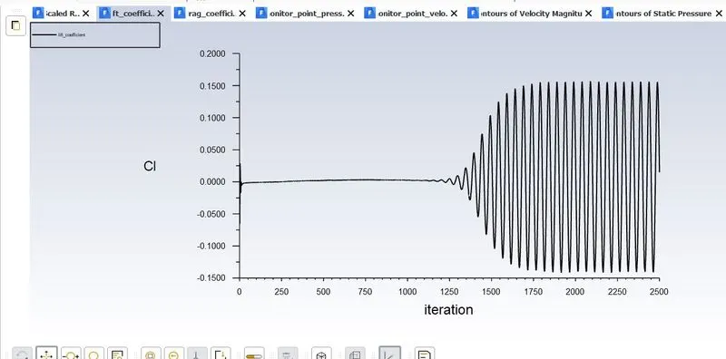
6. Contour of Velocity Magnitude
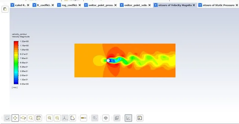
7. Contour of Static Pressure
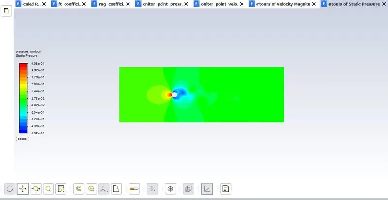
8. Velocity Contour Animation
8. Pressure Contour Animation
9. Strouhal Number
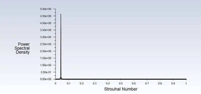
St=0.01
2.
Transient flow over Circular Cylinder at Reynolds number 100
Setting Up the Reynolds Number
Re,d=ρ*U*d/µ
Re,d=100
density=1 kg/m^3
d=2m
µ=0.02 kg/ms
U=1m/s
1. Scaled Residuals
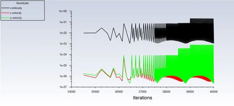
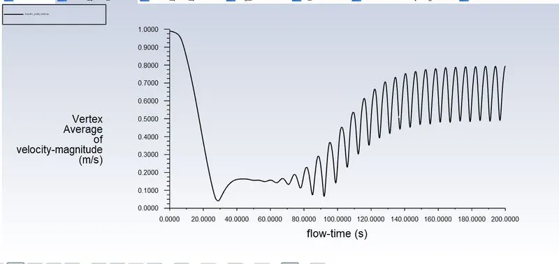
2.Vortex Average of velocity
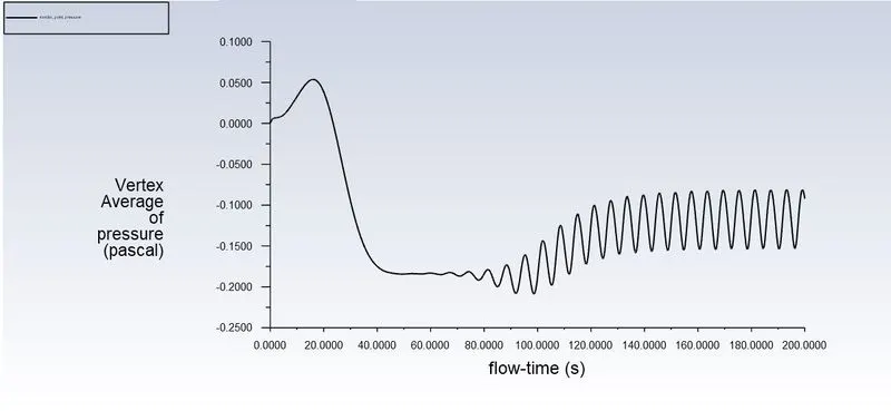
3. Vortex Average of Pressure
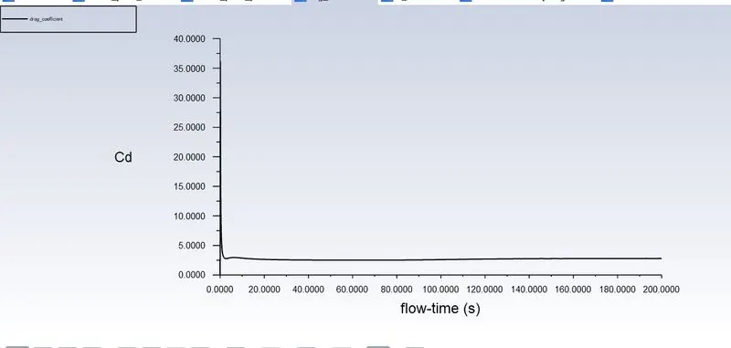
4. Drag Coefficient
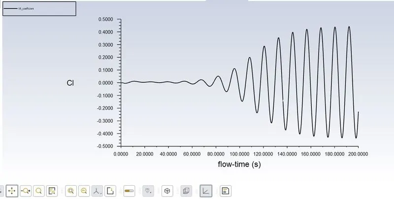
5. Lift Coefficient
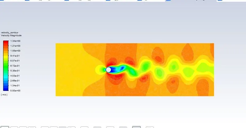
6. Velocity contour
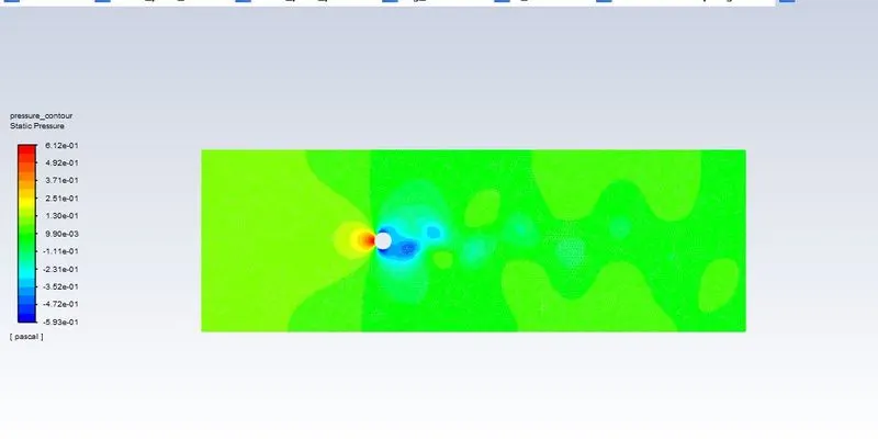
7 Pressure Contour
8. Strouhal Number
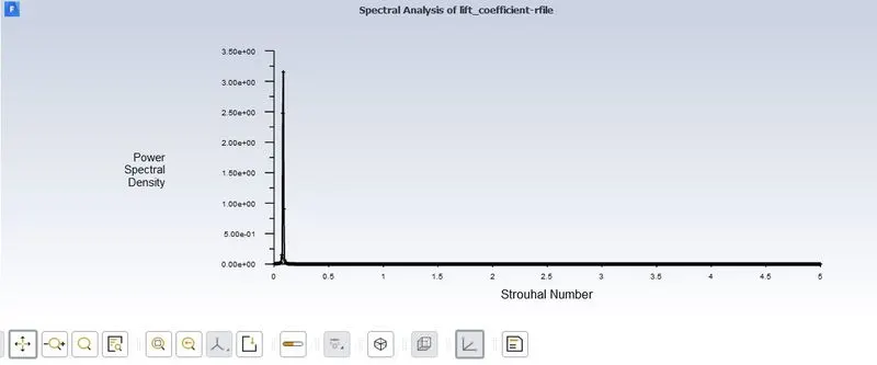
St=0.02
9. Velocity Contour Animation
Symmary of results of part 1
| Reynolds number | Solver | Viscosity (Pa*s) | Velocity (m/s) | Strouhal Number |
| 100 | Steady | 0.02 | 1 | 0.01 |
| 100 | Transient | 0.02 | 1 | 0.02 |
Part 2: Steady flow over circular cylinder at Varying Reynolds number to estimate the fluctuation of Coefficient of Drag and Coefficient of Lift
1. At Re =10 the estimation of Cd and Cl with steady solver
Re,d=ρ*U*d/µ
Re,d=10
density=1 kg/m^3
d=2m
µ=0.02 kg/ms
U=0.1m/s
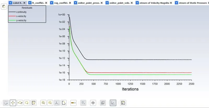
1. Scaled Residuals
2. Coefficient of Lifit
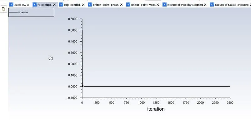
Cl=0.0013726253
3. Coefficient of Drag
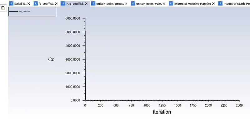
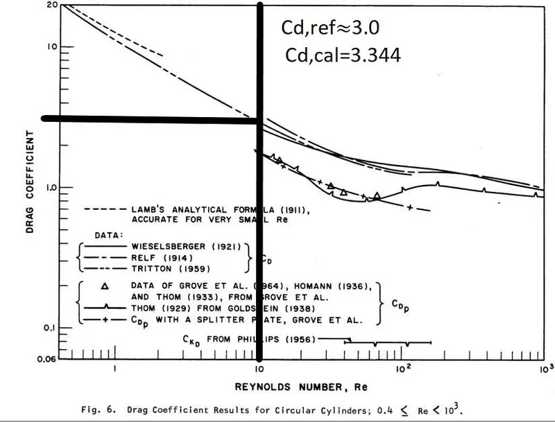
Cd=3.3440213
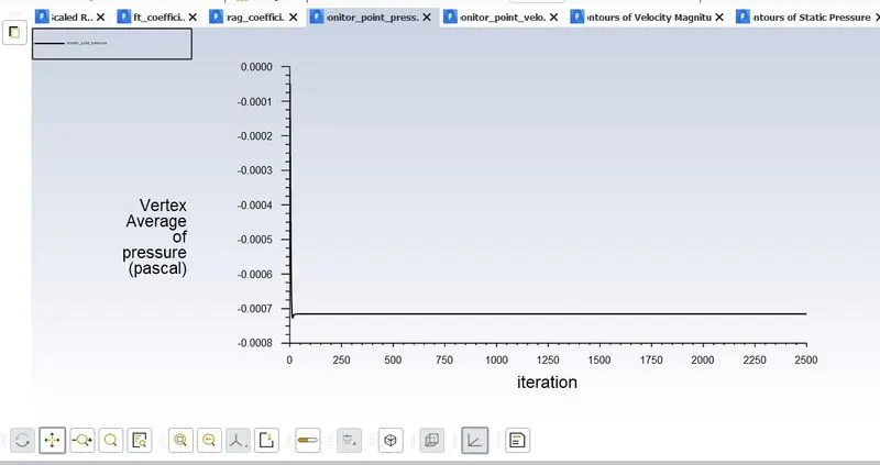
4. Vortex Average of pressure
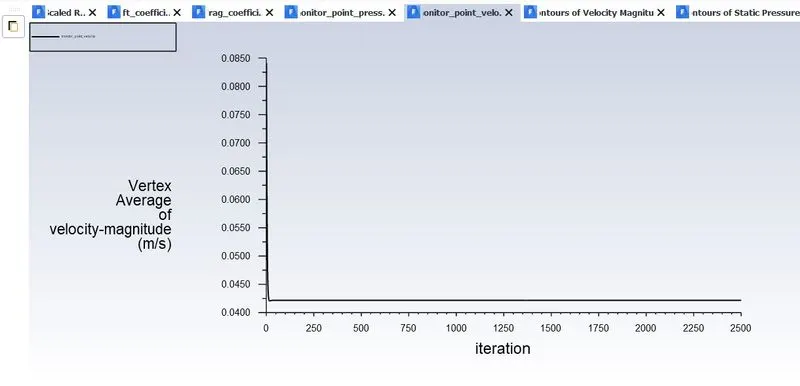
5. Vortex Average of Velocity
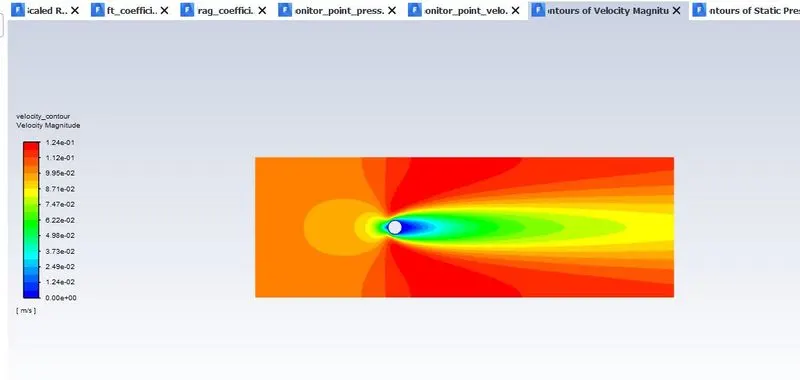
6. Contour of Velocity
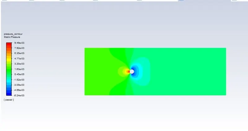
7. Contour of Pressure
2. At Re =100 the estimation of Cd and Cl with steady solver
Re,d=ρ*U*d/µ
Re,d=100
density=1 kg/m^3
d=2m
µ=0.02 kg/ms
U=1m/s
1. Scaled Residuals
2. Vortex average of velocity
3. Vortex Average of pressure
4. Coefficient of Drag
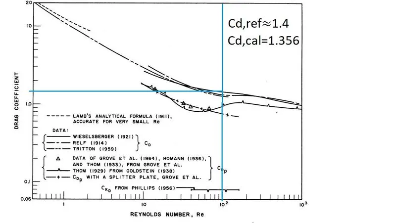
Cd=1.35593
5. Coefficient of lift
Cl (uplift)=0.15 Cl(downlift)=-0.15
6. Contour of Velocity
7.Contour of Pressure
8. Velocity Contour Animation
3. At Re =1000 the estimation of Cd and Cl with steady solver
Re,d=ρ*U*d/µ
Re,d=1000
density=1 kg/m^3
d=2m
µ=0.02 kg/ms
U=10 m/s
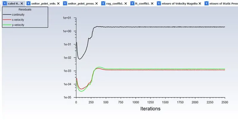
1. Scaled Residuals
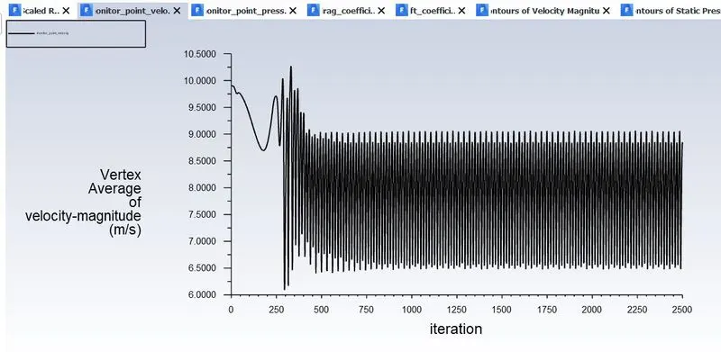
2. Vortex Average of Velocity
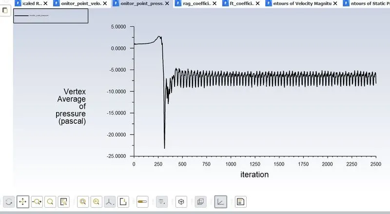
3. Vortex Average of pressure
4. Coefficient of Drag
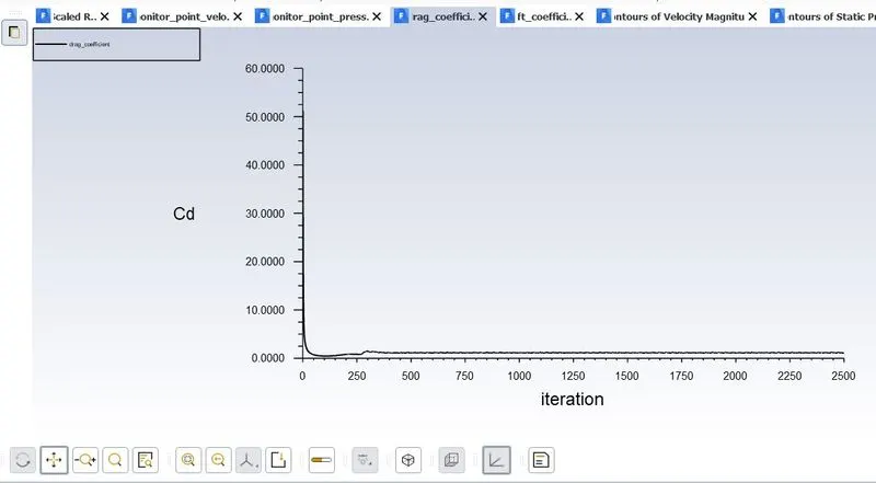
Cd=1.1260374
5. Coefficient of Lift
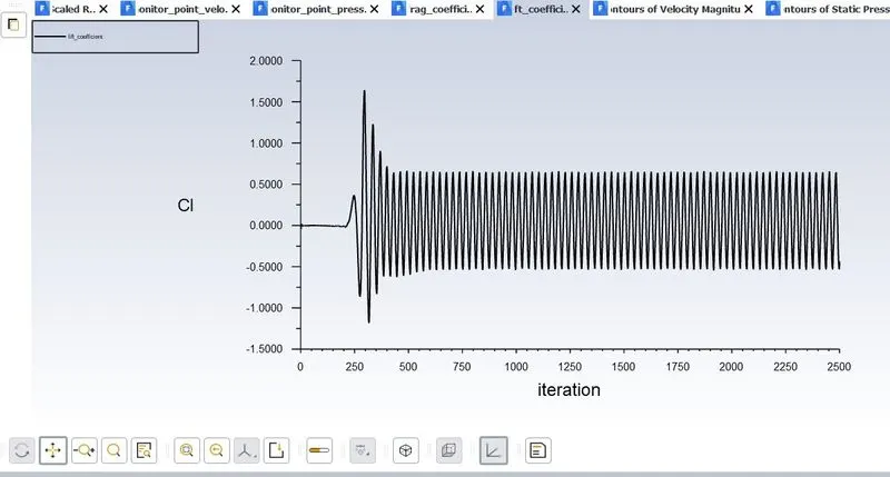
Cl (uplift)=0.7 Cl(downlift)=-0.7
6. Contour of Velocity Animation
3. At Re =10000 the estimation of Cd and Cl with steady solver
Re,d=ρ*U*d/µ
Re,d=10000
density=1 kg/m^3
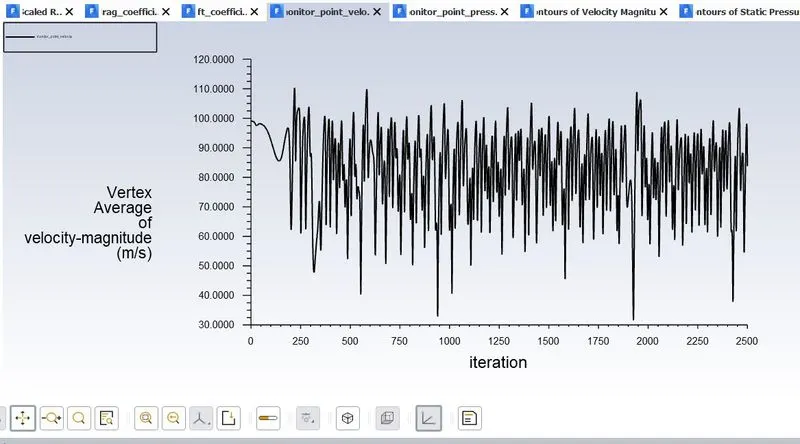
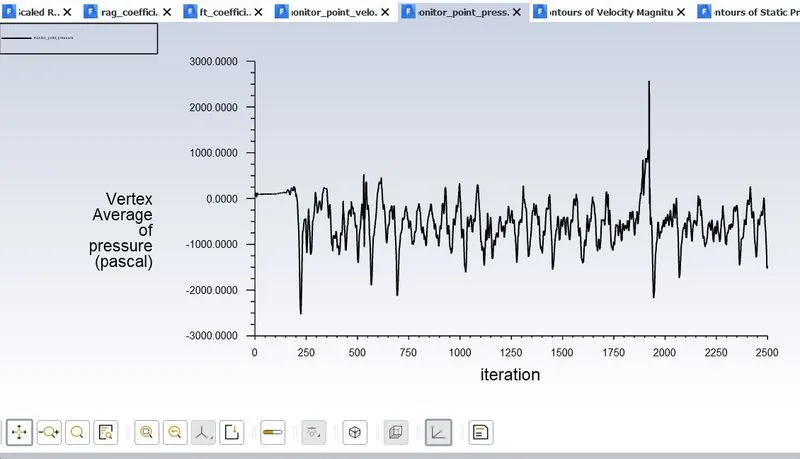
d=2m **Since we are limited to incompressible solver, setting up of viscosity to 0.02 leads to a velocity of 100 m/s and due to vorticity it at times go beyond the
µ=0.02 kg/ms Compressibility limit leading to errors in computation. So, viscosity is reduced here.
U=100m/s
1. Scaled Residuals
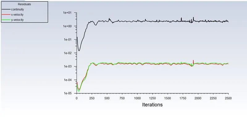
2. Vortex average of Velocity
3. Vortex Average of Pressure
4. Coefficient of Drag
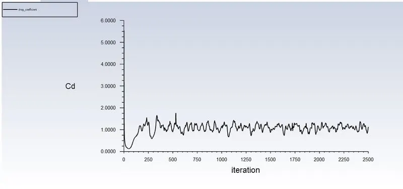
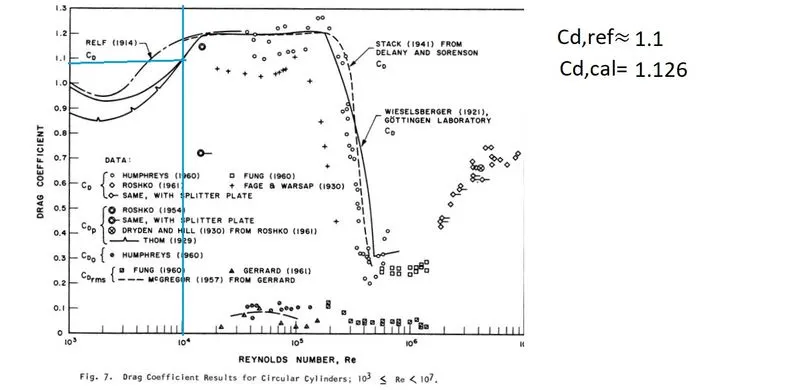
Cd=1.12559
5. Coefficient of Lift
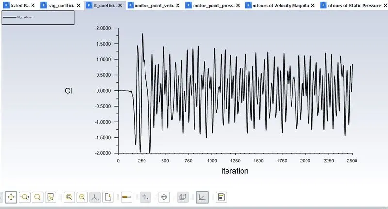
Cl(uplift)=1.5 Cl(downlift)= -1.5
6. Velocity Contour Animation
4. At Re =100000 the estimation of Cd and Cl with steady solver
Re,d=ρ*U*d/µ
Re,d=100000
density=2 kg/m^3
d=2m **Since we are limited to incompressible solver, setting up of viscosity to 0.02 leads to a velocity of 1000 m/s which goes beyond the
µ=0.002 kg/ms Compressibility limit leading to errors in computation. So, viscosity is reduced here.
U=50m/s
1. Scaled Residuals
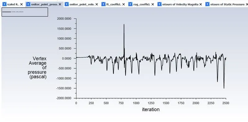
2. Vortex magnitude of velocity
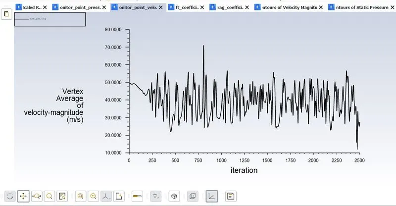
3. Coefficient of Lift
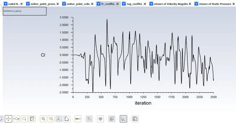
Cl = -1.622707
4. Coefficient of Drag
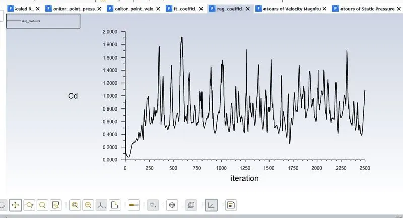
Cd = 1.0790085
5. Contour of Velocity
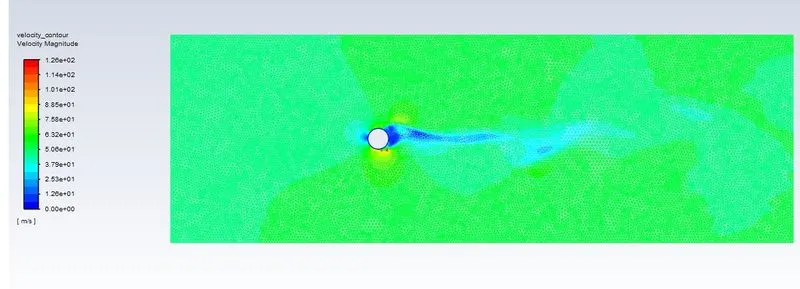
5. Velocity Contour Animation
Summary of Results
| Reynolds Number | Viscosity (Pa*s) | Velocity(m/s) | Cd | CL(uplift) | CL(downlift) | CL |
| 10 | 0.02 | 0.1 | 3.34402 | 0.001373 | ||
| 100 | 0.02 | 1 | 1.35593 | 0.15 | -0.15 | |
| 1000 | 0.02 | 10 | 1.126037 | 0.7 | -0.7 | |
| 10000 | 0.02 | 100 | 1.12559 | - | - |
0.84934626 |
| 100000 | 0.002 | 100 |
0.95448 |
- | - |
0.8832135 |
*Due to turbulent wake after Re>300, the Coefficient of lift also fluctuates very ranndomly.
Validation of Results
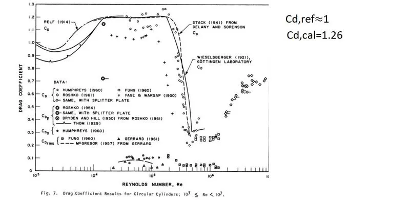
Values of Cd at various Reynolds number taken when frontal area of projection is considered.
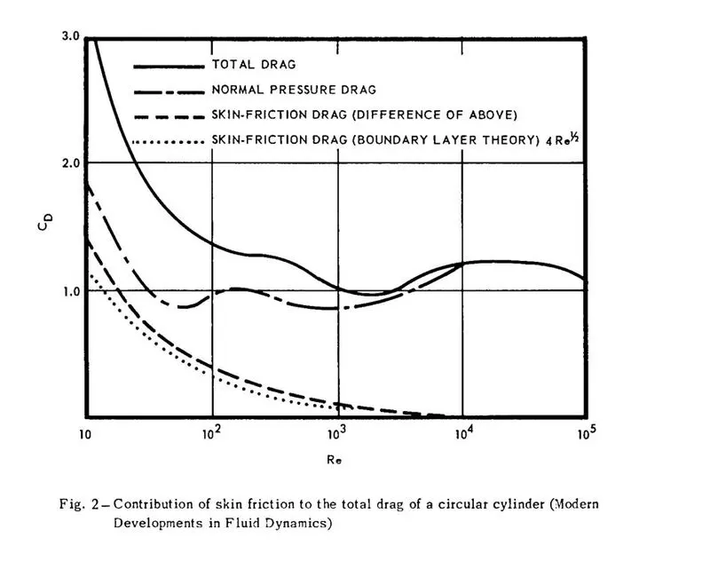 [4]
[4]
1. Re=100
2. At Re=100
3. At Re=1000
4. At Re=10,000
5. At Re=100,000
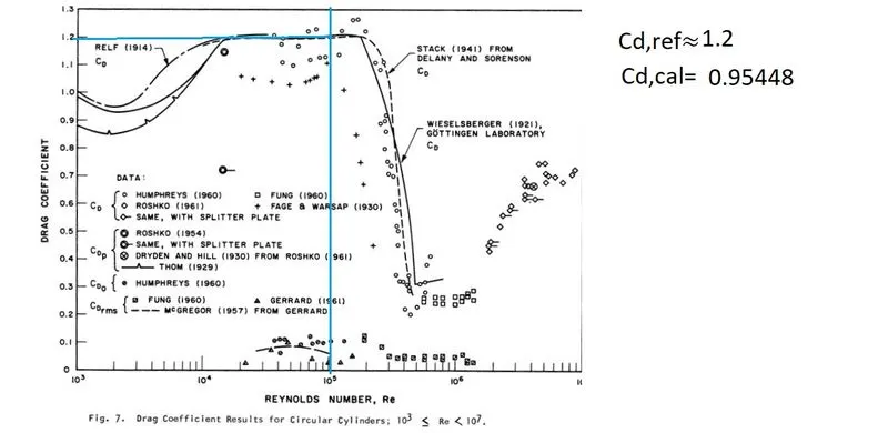
***The results closely resonates with experimental data.
Conclusion:
-
For the transient and steady solver, the strouhal number was close to 0.02.
- The only hydrodynamic force upto Re=40 is Drag, this is because the wake is symmetric and Cl is negligible. As Vortex shedding starts at Re>90, due to periodiciity of vortex shedding the coefficient of lift fluctuates between a max and a min around the mean value of 0. As transition to turbulence occurs, the wake is randomly behaving now and the Coefficient of lift is also fluctuating randomly along with the Coefficient of Drag.
-
At Reynolds number of 10, there was no oscillation of the wake and no vortex shedding. The drag coefficient was high Cd=3.344 and about 43% of this drag is contributed by the skin friction Drag [4]. Thus Fd,f = 1.4379 and Fd,p = 1.9061.
- As Reynolds number reaches 100, we observed a setting up of periodic oscillation of the wake which contributed to the interaction of the seperated boundary layers and consequently, vortex shedding at a regular freaquency emerged. Since the centre of vortex is a region of low pressure, and an accululation of such regions in the wake reduces the pressure there, thus results in the increment of Form Drag on the cylinder. Cd=1.35593, as per the reference [3] 90% of this drag is due to Pressure/form drag. So, Fd,p=1.22 and Fd,f=0.13559.
- 150<Re<300, is the region of turbulence transition in the wake and is very diificult to simulate properly. After Reynolds number surpasses 300, the wake is fully turbulent and no periodicity or regular vortex shedding can be seen, the vortex shedding occurs very abruptly causing fluctuations to both Cd and CL.
- At Re=1000, the wake become narrower, this reults in further reduction of drag, and no regular pattern can be seen in the vortex shedding. Cd=1.1260374 and Cl was fluctuating between 0.7 to -0.7.
- At Re=10000, the Cd remained nearly same although as per the literature a slight increase was expected due to widening of the wake, since our selection of viscosity and velocity brought us very close to the compressibility limit and our use of a Pressure based solver might be the cause of this discripency.
- At Re=100000, the viscosity is such which will set up the velocity unrealistically high thus we reducued the viscosity by a 1/10 and our Cd=0.9544.
- Thus the coefficient of drag was initially very high at low reynolds number due to a wide wake. As Reynolds number is increased a narrowing of wake is observed and a reduction of Cd is observed. At Re=100, the Reynolds number was close to 1, it stick closer to 1, until Re=100000. A very interesting occurance occurs as Re>2*10^5 saperation of flow is delayed as turbulence occurs prior to seperation wake is narrowed and Cd is at its lowes =0.3, this phenomena is called Drag Crises and can be studied with proper turbulence modelling.\
Referance
2. Synopsis for lift, drag and vortex freaquency data for regid circular cylinders-John. H. Lenhard 1966.
3. www.aerodynamics4students.com
4. Symmary of Drag and Lift coefficients for various shaed Cylinders, Heddleson, Brown, Cliffe, General Electric 1957
5. https://demonstrations.wolfram.com/ProjectedAreasofCylinderAndCone/