Week 2 - Flow over a Cylinder.

FLOW OVER A CYLINDER

AIM: To stimulate the flow over a cylinder for two different cases to understand the phenomenon of the Karman vortex.

OBJECTIVE:

To Use the steady and unsteady solver for the first case. For the second case use the steady solver for different Reynolds number to study the phenomena of the Karman vortex in both cases.

CASE-I

1. Simulate the flow with the steady and unsteady case and calculate the Strouhal Number for Re= 100.

CASE-II

1. Calculate the coefficient of drag and lift over a cylinder by setting the Reynolds number to 10,100,1000,10000 & 100000. (Run with steady solver)
2. Discuss the effect of Reynolds number on the coefficient of drag. [ Results should be validated with any standard literature and error should be within 5 %]

Expected results: -

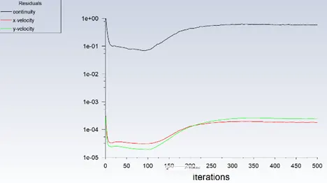
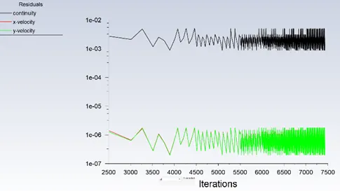
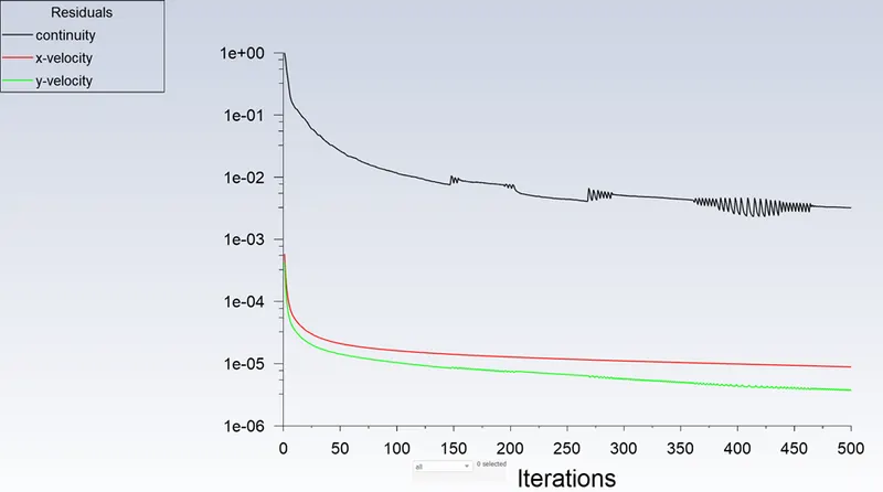
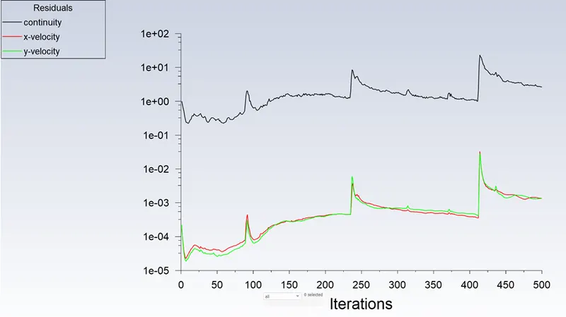
1. In both approaches, show that the flow has converged. That is, what quantities or plots need to be looked at to determine that the flow has converged?
2. Plots of the coefficient of drag and lift.
3. Plots to show vortex shedding behind the cylinder.
4. Mention the referred material (Reference Paper or Fluid Mechanics Textbook) at the end of the challenge submission page.

INTRODUCTION:

Flow over a cylinder is important in many industrial applications like cooling of iron or cylindrical pipe. Circular pipes have more application in heat exchanger. High temperature flue gases flow over a circular cylinder in a cross flow. Depending on flow rate, fluid properties and size of cylinder, the flow can be laminar, transition and turbulent. External flows past objects have been studied extensively because of their many practical applications. For example, airfoil are made into streamline shapes to increase the lifts, and at the same time, reducing the aerodynamic drags exerted on the wings. On the other hand, flow past a blunt body, such as a circular cylinder, usually experiences boundary layer separation and very strong flow oscillations in the wake region behind the body. In certain Reynolds number range, a periodic flow motion will develop in the wake because of boundary layer vortices being shed alternatively from either side of the cylinder. This regular pattern of vortices in the wake is called a Karman vortex street. It creates an oscillating flow at a discrete frequency that is correlated to the Reynolds number of the flow.

STROUHAL NUMBER

In dimensional analysis the Strouhal number (St, or sometimes Sr to avoid the conflict with the stanton number) is a dimensionless number describing oscillating flow mechanisms. The parameter is named after Vincent strouhal, a Czech physicist who experimented in1878 with wires experiencing vortex shedding and singing in the wind. The Strouhal number is an integral part of the fundamentals of fliud mechanics.

The Strouhal number is often given as

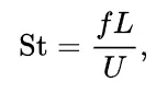
where f is the frequency of vortex shedding, L is the characteristic length (for example, hydraulic diameter) and U is the flow velocity. In certain cases, like heaving (plunging) flight, this characteristic length is the amplitude of oscillation. This selection of characteristic length can be used to present a distinction between Strouhal number and reduced frequency:

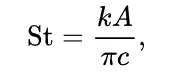
where k is the reduced frequency and A is amplitude of the heaving oscillation.

REYNOLDS NUMBER

The Reynolds number is defined as

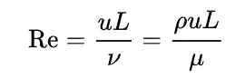
where:

• ρ is the density of the fluid (SI units: kg/m³)
• u is the flow speed (m/s)
• L is a characteristic linear dimension (m) (see the below sections of this article for examples)
• μ is the dynamic viscosity of the flui (Pa·s or N·s/m² or kg/(m·s))
• ν is the kinematic viscosity of the fluid (m²/s).

Co-efficient of Drag

The drag coefficient cd is defined as

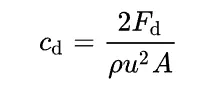
where:

• F_d is the drag force, which is by definition the force component in the direction of the flow velocity.
• ρ is the mass density of the fluid,
• u² is the flow speed of the object relative to the fluid.
• A is the reference area

Co-efficient of Lift

The lift coefficient C_L is defined by

where,

• L is the lift force,
• S is the relevant surface area.
• q is the fluid dynamic pressure,
• ρ is the mass density of the fluid,
• u² is the flow speed of the object relative to the fluid.

Steps involved in analysis:

• Pre-processing
• Solving
• Post-processing

CASE 1:

• Simulate the flow with the steady and unsteady case and calculate the Strouhal Number for Re= 100.

Pre-processing:

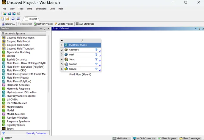
• From the analysis system toolbox open the Fluid Flow (Fluent)

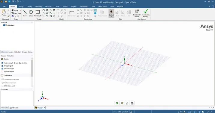
• In Geometry open the spaceclaim for the 2D designing of the model.

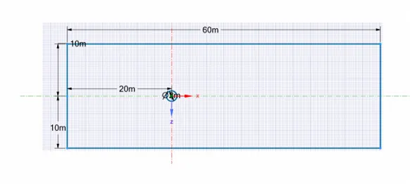
• Geometry of the model is designed and extract using pull tool.

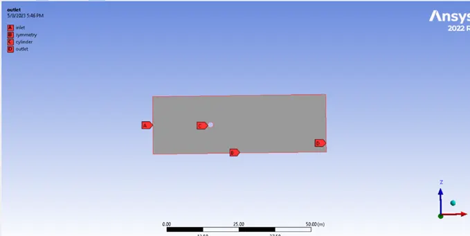
• Close the spaceclaim and go to mesh. Create the named selection to the model.

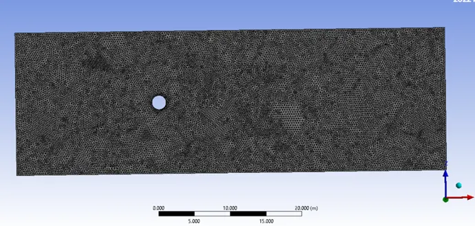
• The triagonal mesh is generated for size of 0.25m.

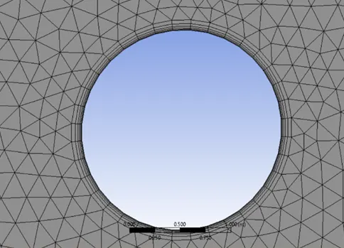
• The inflation up to 6 layers is given around the cylinder to capture the flow over it.
• Solving:
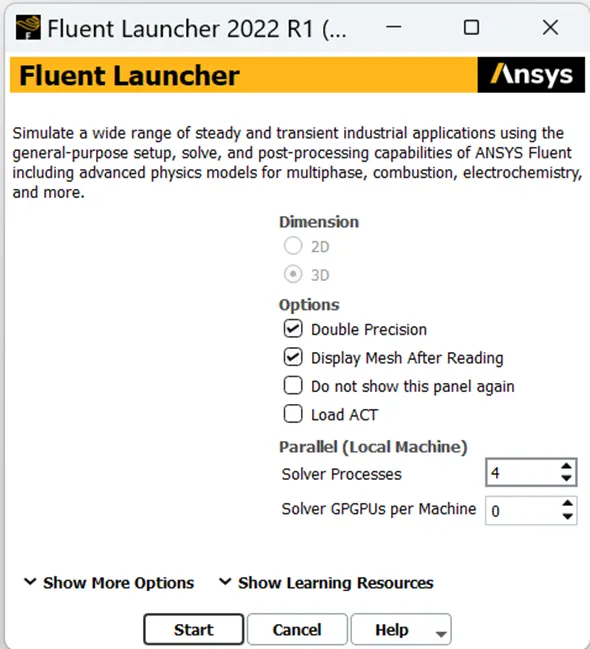
• Open the setup for applying the boundary condition for the fluid flow solution.

Setup	LAMINAR	LAMINAR
Solver time	Steady state	Un-Steady state
Solver type	Pressure Based	Pressure Based
Viscous Model	LAMINAR	LAMINAR
Material	Air o Density- 1kg/m3 o Viscosity – 0.02 Pa s	Air o Density- 1kg/m3 o Viscosity – 0.02 Pa s
Boundary Condition	Inlet Velocity-1m/s Outlet Pressure Outlet Wall No slip wall. Stationary wall	Inlet Velocity-1m/s Outlet Pressure Outlet Wall No slip wall. Stationary wall

• Scaled residual plots.

STEADY-STATE	UNSTEADY-STATE

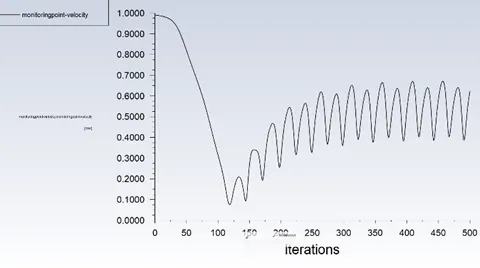
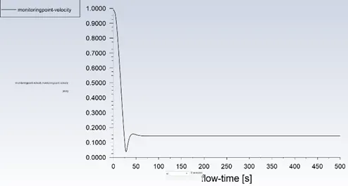
• Vertex average plots at monitoring points.

STEADY-STATE	UNSTEADY-STATE

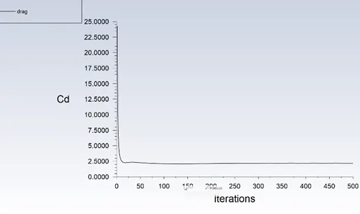
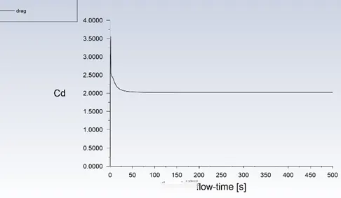
• Co-efficient of Drag plots.

STEADY-STATE	UNSTEADY-STATE

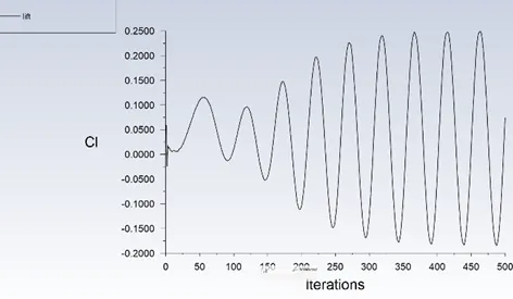
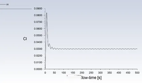
• Co-efficient of lift plots.

STEADY-STATE	UNSTEADY-STATE

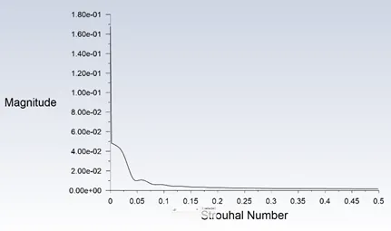
• Strouhal Number plots.

STEADY-STATE	UNSTEADY-STATE
'Not possible in the steady state’

• Post-processing:
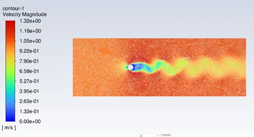
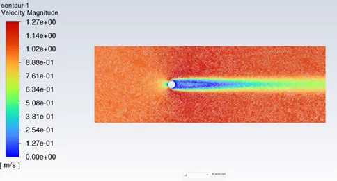
• Velocity contour

STEADY-STATE	UNSTEADY-STATE

Conclusion

The results of the steady and unsteady case and calculated the Strouhal Number for the Reynolds number (Re= 100). Below are the result values.

Solver type	Coefficient of drag	Coefficient of lift	Monitoring point-velocity(m/s)	Strouhal number
Steady State	1.364185	0.07834064	0.62	-
Unsteady State	1.487127	0.02974656	0.14	0.1157

CASE 2:

• Calculate the coefficient of drag and lift over a cylinder by setting the Reynolds number to 10,100,1000,10000 & 100000. (Run with steady solver)

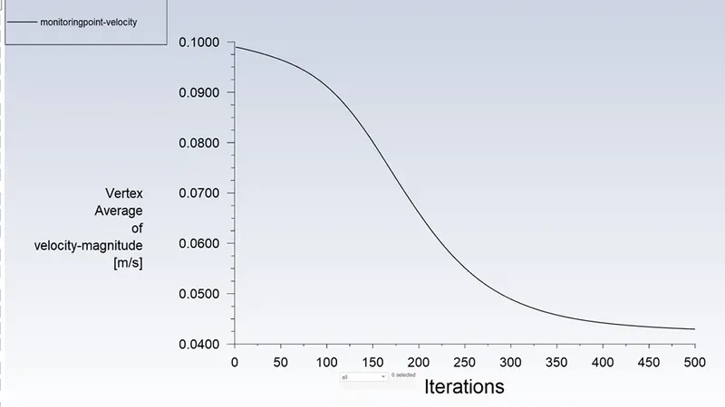
Steady state with condition Re = 10

Residual Plot:

Vertex at monitoring point Plot:

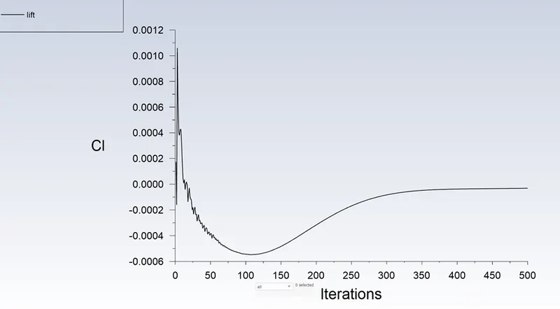
Coefficient of Lift Plot:

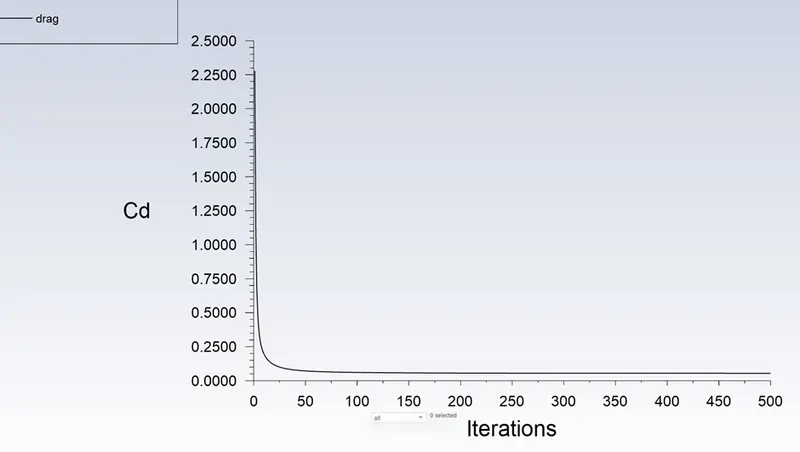
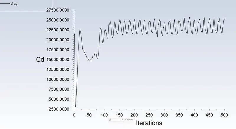
Coefficient of Drag Plot:

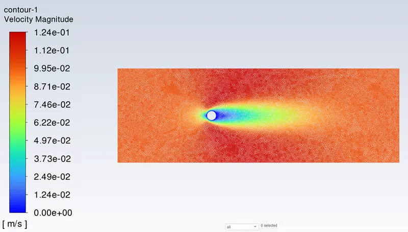
Velocity Contour:

Steady state with condition Re = 100

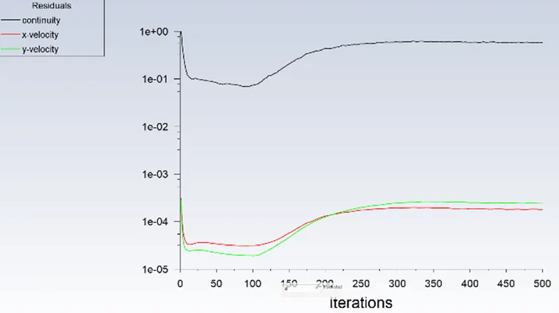
Residual Plot:

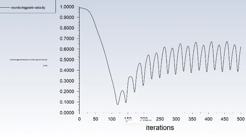
Vertex at monitoring point Plot:

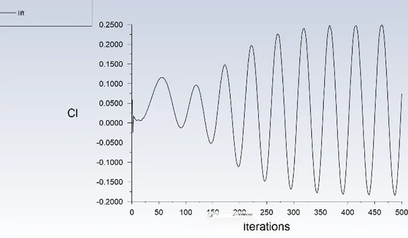
Coefficient of Lift Plot:

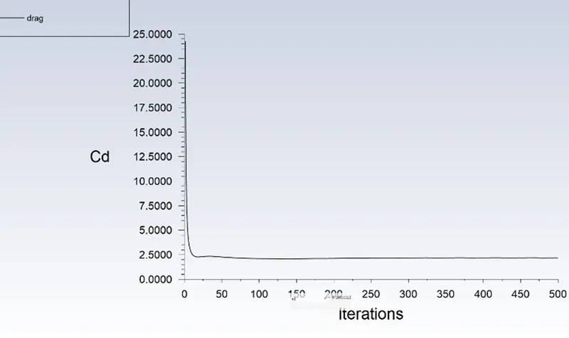
Coefficient of Drag Plot:

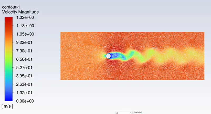
Velocity Contour:

Steady state with condition Re = 1000

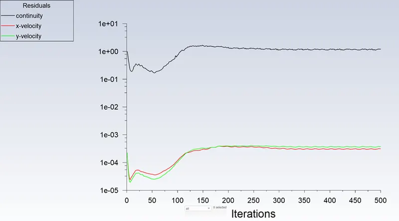
Residual Plot:

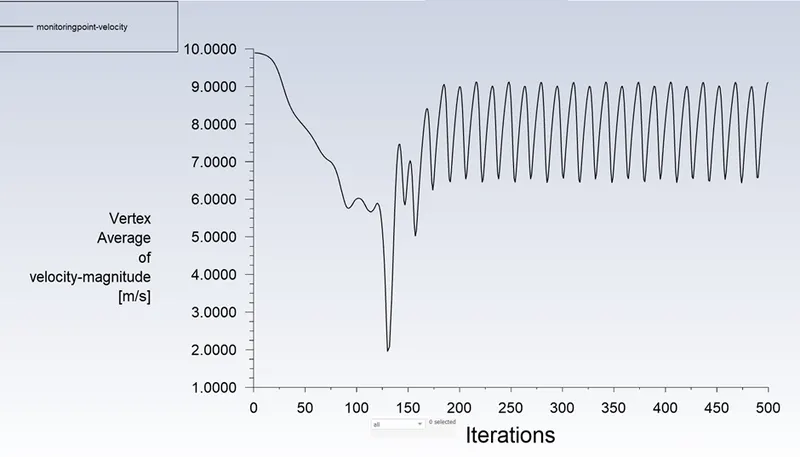
Vertex at monitoring point Plot:

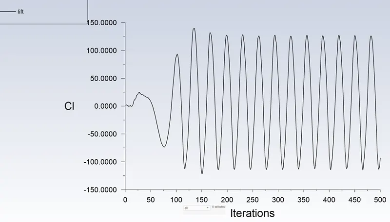
Coefficient of Lift Plot:

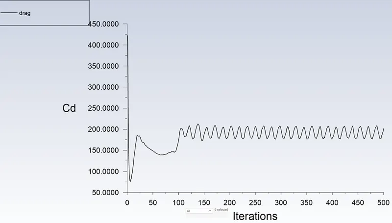
Coefficient of Drag Plot:

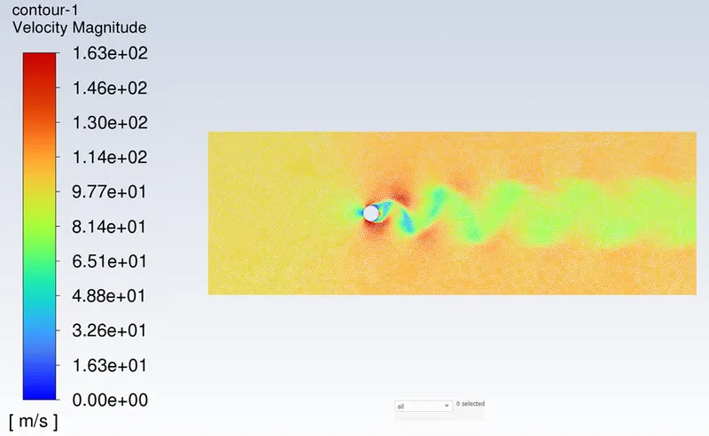
Velocity Contour:

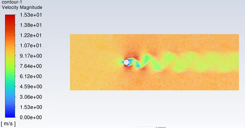
Steady state with condition Re = 10000

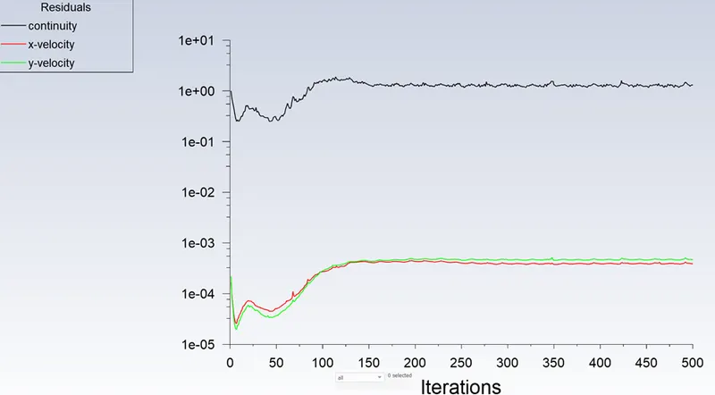
Residual Plot:

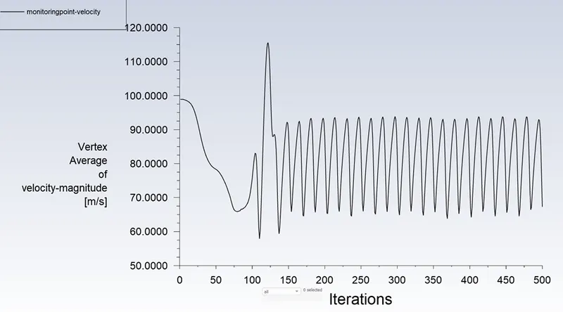
Vertex at monitoring point Plot:

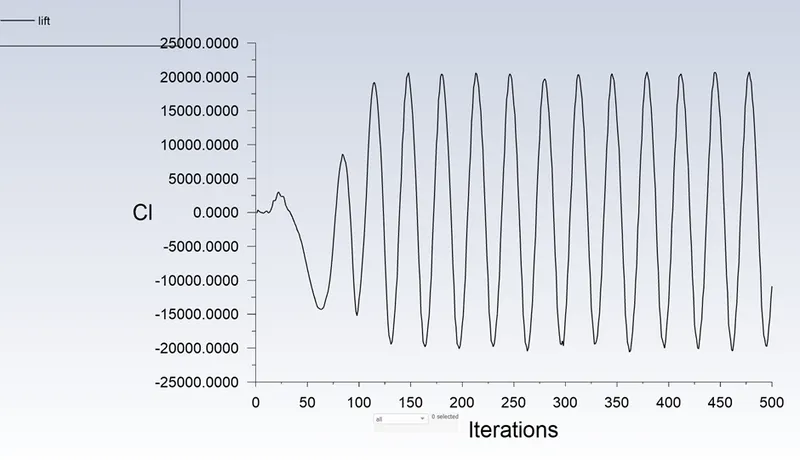
Coefficient of Lift Plot:

Coefficient of Drag Plot:

Velocity Contour:

Steady state with condition Re = 100000

Residual Plot:

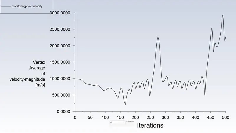
Vertex at monitoring point Plot:

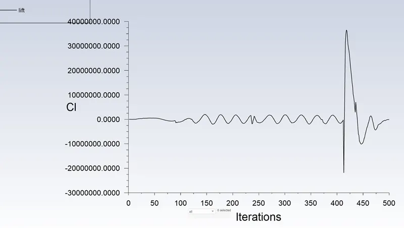
Coefficient of Lift Plot:

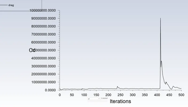
Coefficient of Drag Plot:

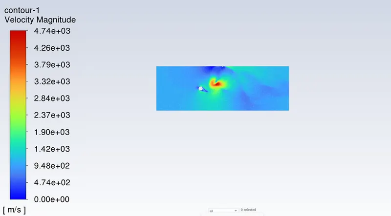
Velocity Contour:

Comparison table:

Reynolds Number	Monitoring point velocity(m/s)
10	0.043
100	0.623
1000	9.10
10000	67.29
100000	2270.79

Conclusion:

• From the results, I conclude that by increasing the Reynolds number drastically we can’t be able to observe the Karman vortex shedding behind the cylinder.
• It results that drag increases and lift decreases drastically, because of two reasons one is blend body and then inlet flow with higher Reynolds number.
• For the case I, we are not calculated the Strouhal number for steady state solver. Because we need flow time for frequency to calculate the Strouhal number.

Reference Paper

• https://www.sciencedirect.com/science/article/pii/S0307904X08000243
• https://en.wikipedia.org/wiki/Strouhal_number
• https://en.wikipedia.org/wiki/Reynolds_number
• https://en.wikipedia.org/wiki/Drag_coefficient
• https://en.wikipedia.org/wiki/Lift_coefficient