Week 2 - Flow over a Cylinder.

AIM

• Simulate the flow with the steady and unsteady case and calculate the Strouhal Number for Re= 100.
• Calculate the coefficient of drag and lift over a cylinder by setting the Reynolds number to 10,100,1000,10000 & 100000 with steady state solver and discuss the effect of Reynolds number on coefficeint of drag
• Plot coefficient of drag and lift.
• Plot vortex shedding behind cylinder.

Theory

Flow around a circular cylinder is essential for researchers and engineering design aspects. Moreover, the flow over the circular cylinders have a wide range of applications such as in heat exchanger, cooling towers, nuclear cooling system, bridge piers, subsea pipelines can be modeled as cylinder. Most of engineering problems are subjected to sub-critical Reynolds number. Boundary layer separation and flow oscillation in the wake zone behind the cylinder occur due to shedding of vortices at moderate and high Reynolds number. These types of flow can sometimes results to undesirable structural vibrations, which leads to structural damage. Therefore, this kind of flow behavior is very interesting to be studied in deeply especially the effects of the vortex shedding on the cylinder.

Reynold Number

The Reynolds number is the ratio of inertial forces to viscous forces within a fluid that is subjected to relative internal movement due to different fluid velocities. It is given by the formula

`Re= (rhoVD)/mu` where,

`rho`- Density of fluid (Kg/`m^3`)

V - Free stream velocity (m/s)

D - Characteristic length of the body (m)

`mu` - Dynamic viscosity of fluid (Kg/ms)

It is used to predict the transition of fluid flow from laminar to turbulent. In boundary layer flow over a flat plate, experiments confirm that, after a certain length of flow, a laminar boundary layer will become unstable and turbulent. This instability occurs across different scales and with different fluids, usually when Re_x ≈ 5×10⁵ , where x is the distance from the leading edge of the flat plate, and the flow velocity is the freestream velocity of the fluid outside the boundary layer. For flow in a pipe of diameter D, experimental observations show that laminar flow occurs when Re < 2300 and turbulent flow occurs when Re > 2900.

Strouhal Number

Strouhal Number is a dimensionless value useful for analyzing oscillating unsteady fluid flow dynamics problems. It is given by the formula

`(St)=(fL)/V` where

f - Oscillation frequency

L - Characterisitc length

V - Free stream velocity

The Strouhal Number can be important when analyzing unsteady, oscillating flow problems. The Strouhal Number represents a measure of the ratio of the inertial forces due to the unsteadiness of the flow or local acceleration to the inertial forces due to changes in velocity from one point to an other in the flow field.

Coefficient of Drag

It is a dimensionless quantity that is used to quantify the drag or resistance of an object in a fluid environment, such as air or water. It is used in the drag equation in which a lower drag coefficient indicates the object will have less aerodynamic or hydrodynamic drag. The drag coefficient is always associated with a particular surface area. The formula is given by

`C_d = (2F_d)/(rhoV^2A` where

`C_d` - Coefficient of drag

`F_d` - Drag force

`rho` - Density of fluid

V - Free stream velocity

A - Crossectional area of body

Coefficient of Lift

It is a dimensionless quantity that is used to determine the lift of a body in the fluid environment. it is given by

`C_L = F_L/((1/2)rhoV^2A)` where,

`C_L` - coefficient of lift

`F_L` - Lift force

`rho` - Density of the fluid

V - Free stream velocity'

A - Cross sectional area of body

Von Karman Vortex Street

Von Karman vortex street is a repeating pattern of swirling vortices, caused by a process known as vortex shedding, which is responsible for the unsteady separation of flow of a fluid around blunt bodies. Vortex shedding is a phenomenon, when the wind blows across a structural member, vortices are shed alternately from one side to the other, and where alternating low-pressure zones are generated on the downwind side of the structure giving rise to a fluctuating force acting at right angles to the wind direction

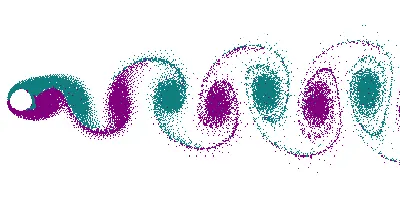
Karman vortex shedding occurs due to the flow separation around the structures. The alternate shedding of vorticity behind the structures leads to periodic pressure oscillations both in the transverse and flow directions.

Procedure

• Our aim is to simulate the flow around a 2D cylinder in steady and unsteady state and calculate the Strouhal number for Reynolds number of 100.
• First we need to create the geometry for analysis.
• Open Spaceclaim in fluent workbench to create the geometry.
• Ensure that the units are in SI. (Length - m)
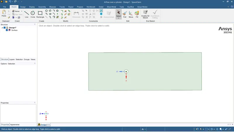
• Draw a circle with diameter of 2 m. A boundary rectangle is created around the circle with distances 10D towards the left of the circle, 20D towards the right of the circle, 5D above and below the circle.
• Use Pull tool to extract the surface from the 2D drawing.
• Close spaceclaim.
• Open mesh module in the fluent workbench. Once you click on the mesh, you can see the default mesh that has been applied to the geometry.
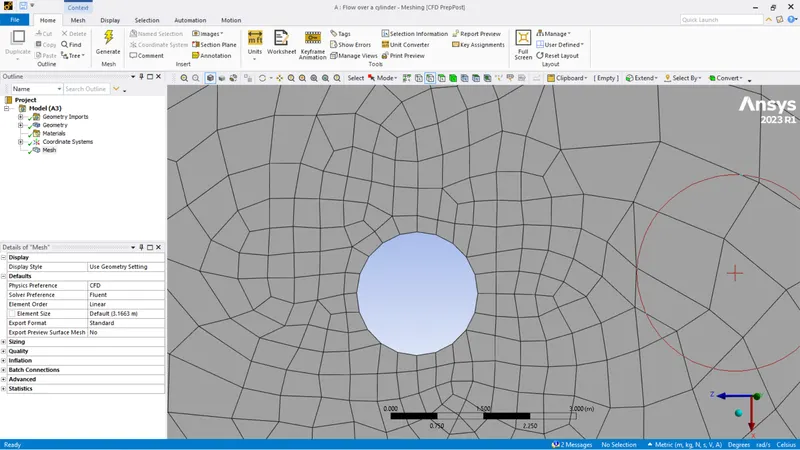
• Upon examination we can see that the mesh is very coarse and the definition of the circle is not proper.
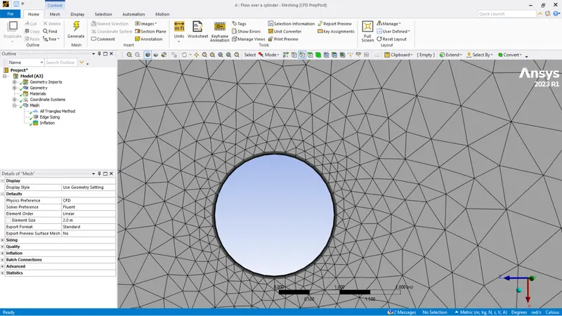
• Rigth click on mesh and insert method>triangles to update the mesh element to triangles.
• You can further refine the mesh by inserting sizing of the circle.
• Inflation layers can be added to the mesh to better capture the geometry. Inflation layers help to accurately capture the results in the bondary region.
• The mesh was updated with the above modifications and mesh element size of 2 m.
• Next we name the parts of the mesh.
• Once the part of the mesh have been appropriately named, we can close the mesh module and move onto the setup.

Simulation of flow over cylinder with Re=100 using steady state solver

• Open the setup with double precision.
• Perform mesh check.

Type	Pressure Based
Time	Steady
Velocity formulation	Absolute
Energy	Deselected because of no temeprature effects
Viscous model	Laminar

We are required to create a user defined material in the material database with denstiy as 1 kg/m3 and dynamic viscosity as 0.02 kg/ms. The dyanamic viscosity was calculated using the Reynolds number equation with a Reynolds number of 100 and velocity at inlet of 1 m/s.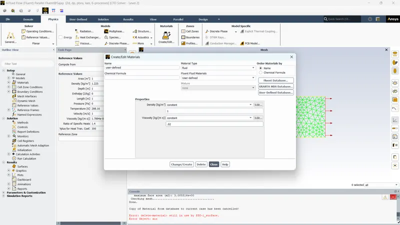

The boundary conditions were given as below

Inlet	Velocity Inlet; Magnitude : 1 m/s
Outlet	Pressure Outlet, Gauge pressure : 0 Pa
Cylinder_Wall	Wall; Stationary; No Slip
Symmetry	Symmetry

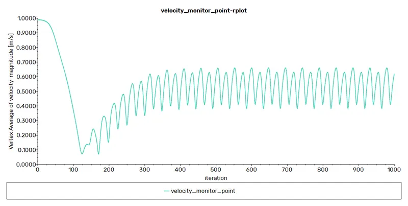
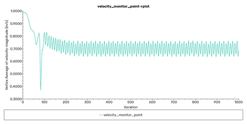
We need to observe the vortex shedding. For this a monitor point for velocity was created at a distance of 4D from the centre of the circle. This is done by moving into the results tab>create>point>coordinates.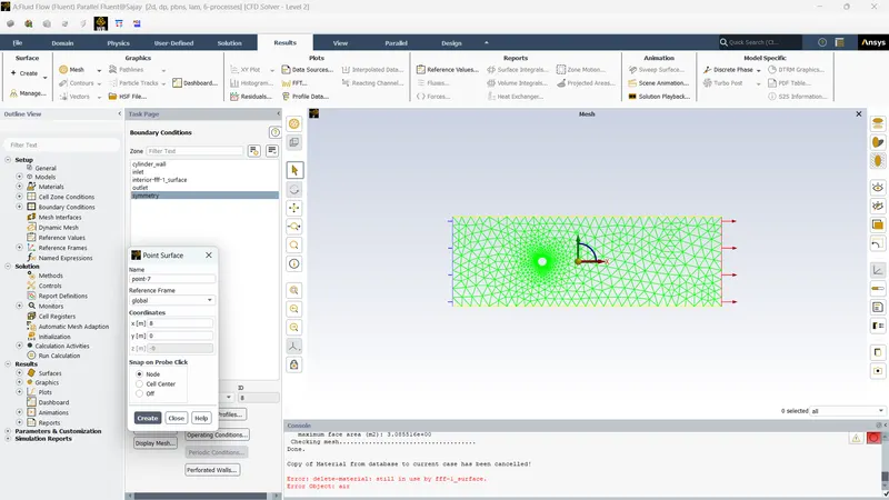

Once monitor point is created, we can plot velocity magnitude at that location using definitions by New>surface>vertex average>monitor point Velocity and give velocity as field variable.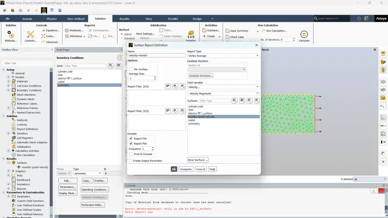

We need to have calculations for the number of iterations that we give. Therefore, we deselect the convergence criteria since the solution can converge before the number of iterations is reached.

The solution method used is SIMPLE algorithm.

Hybrid initialization is done and velocity and pressure contours are created using results tab>contours.

The calculation is done for 500 iterations.

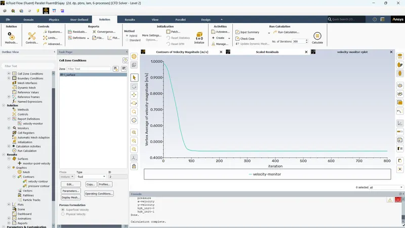
The vortex shedding was not observed even after 800 iterations. Mesh refinement has to be done. The element size of the mesh was reduced gradually and the same setup mentioned above was used to run the simulation.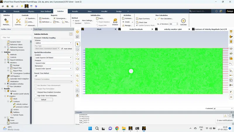

At mesh element size of 0.25 m, we can see the vortex shedding properly. Solution>activities>create>solution animation can be used to create the animation of the velocity contour. The solution was run for 500 iterations.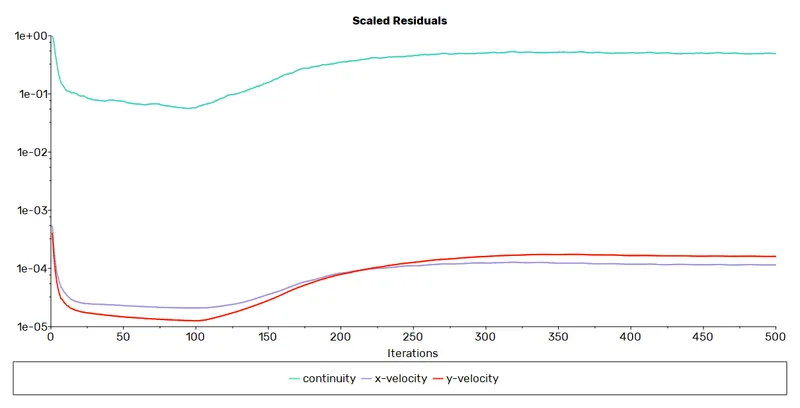

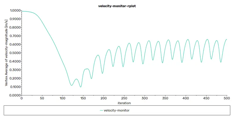
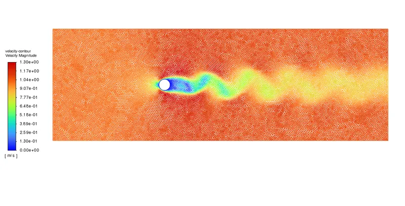
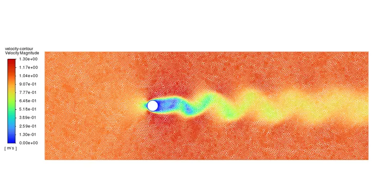
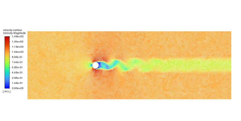
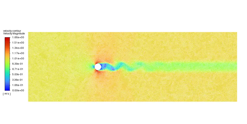
The above images show the vortex shedding happening downstream of the cylinder when the Reynolds number is 100.

Since we are doing the simulation in steady state, we cannot calculate Strouhal number since we need to know the frequency of vortex shedding. To find frequency, we need to do the simulation in transient state.

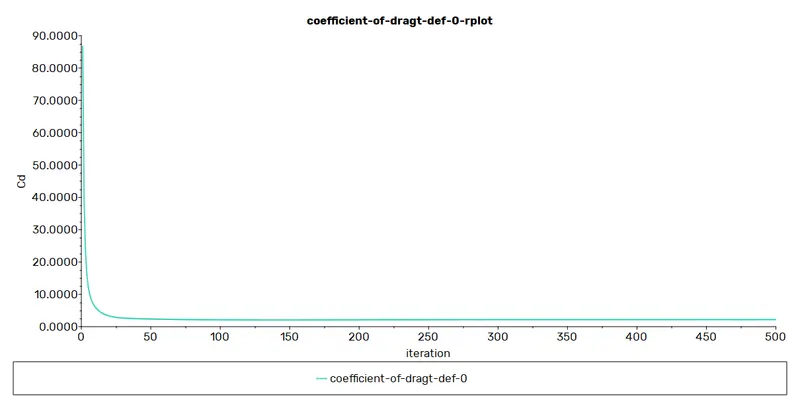
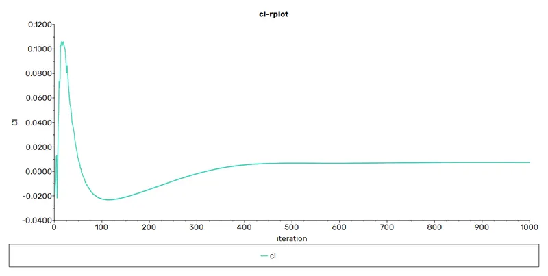
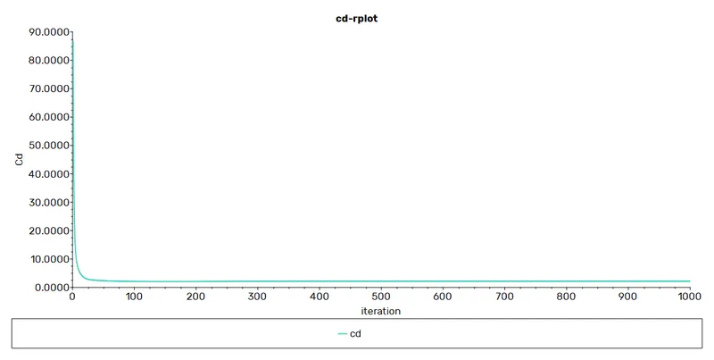
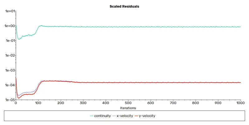
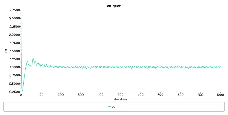
From the residuals plot and coefficeint of drag plot, we can observe that the solution is having a steady value, so we can conclude that the solution is converged.

Simulation of flow over cylinder with Re=100 using Transient state solver

The same setup conditions and boundary conditions were used for the simulation except steady state solver was changed to transient simulation with a time step size of 0.1 s and number of time steps 2000, i.e., for 200 s.

The solution was initialized using standard initialization and the solution was calculated. The result are as follows

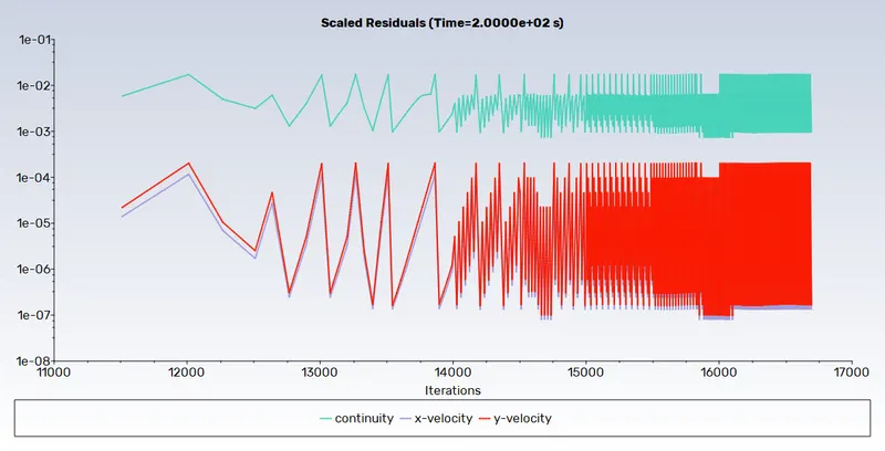
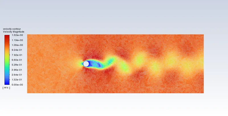
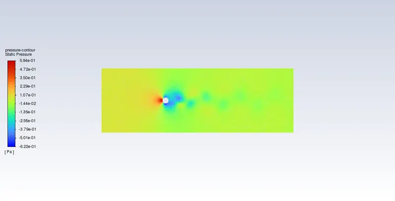
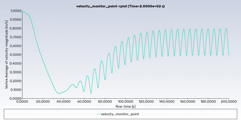
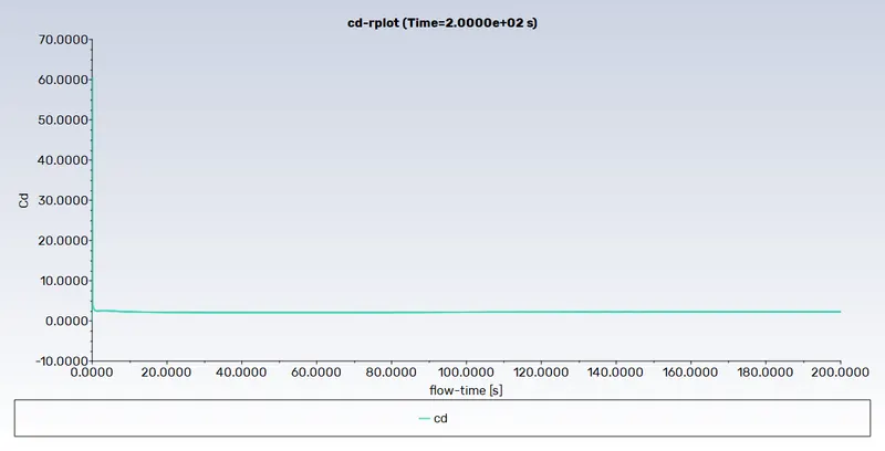
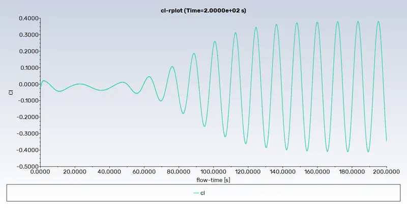
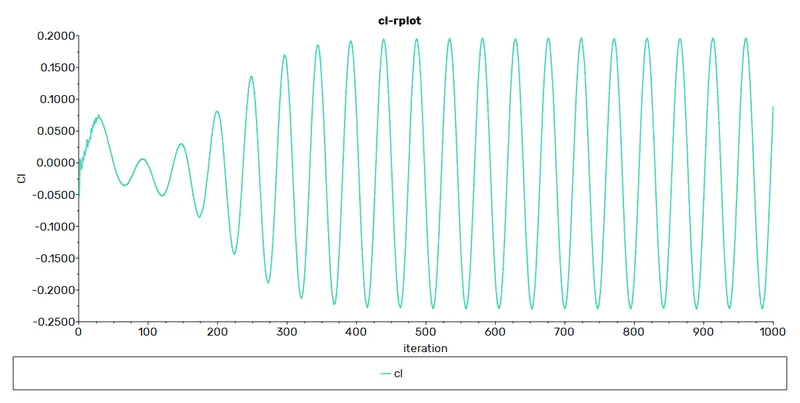
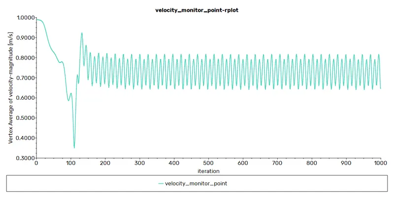
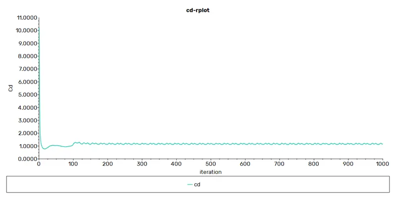
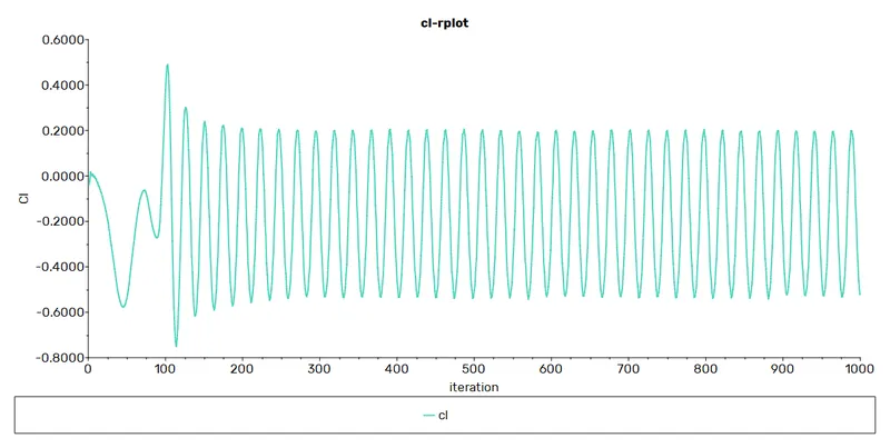
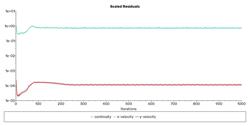
From the constant fluctuating of residuals and steady value of coefficeint of drag, we can conclude that the solution has converged.

We can use FFT to calculate Stroual number from velocity monitor point.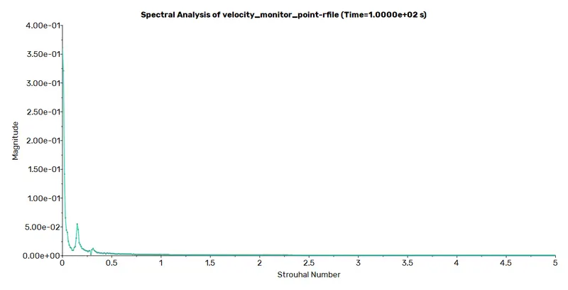

From the graph, the Strouhal number was calculated to be 0.143

Alternatively, we can fid the frequency of the vortex shedding from the velocity magnitude v/s time graph and calculate the Strouhal number from the formula St=fL/v. The time period between two peaks of velocity fluctuation is approximately 7 seconds. So the frequency would be f=1/7= 0.1428. Substituting this in the Strouhal Number equation gives us a value of 0.1428.

Case 2

Reynolds Number = 10

Density = 1 kg/m3

Inlet Velocity = 1 m/s

->Dynamic viscosity = 0.2 Kg/ms

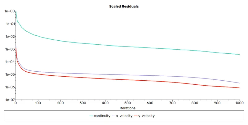
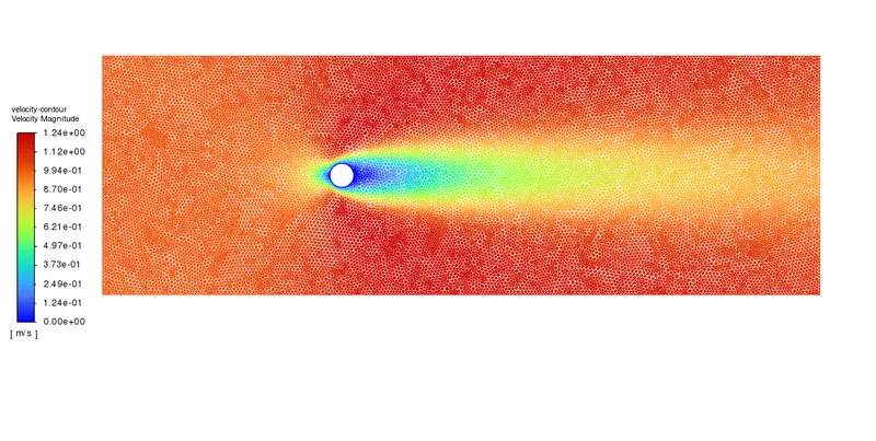
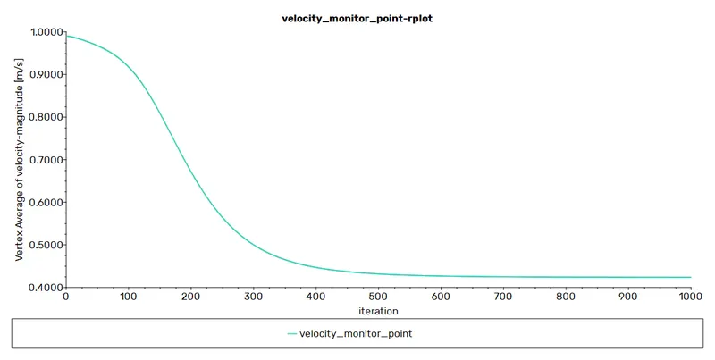
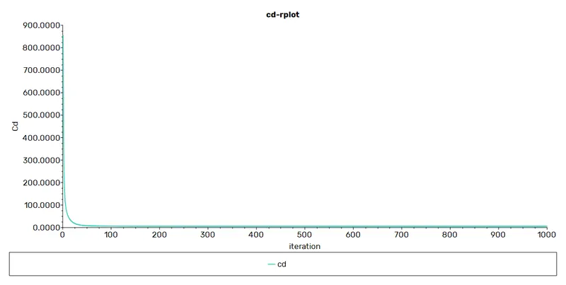
Update the fluid property in the matrials. Run Steady state simulation with hybrid initialization for 1000 iterations.

Reynolds number = 100

Dyanamic Viscosity = 0.02 kg/ms

Update the material property and run the simulation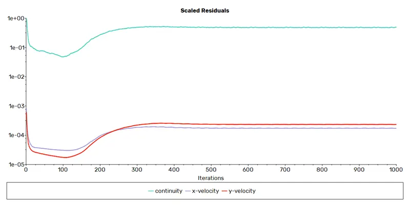

Reynolds number = 1000

Dynamic Viscosity = 0.002 kg/ms

Update the material and run the simulation

Reynolds number = 10000

Dynamic viscosity = 0.0002 kg/ms

The materail property was updated and the simulation was run for 1000 iterations using hybrid initialization.

Reynolds Number = 100000

Dynamic viscosity = 0.00002 Kg/ms

Update the material property and run the simulation for 1000 iterations using hybrid initialization.

Result

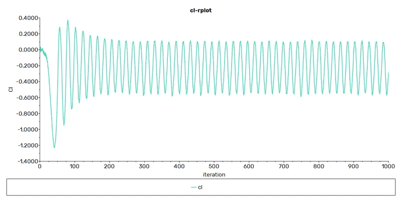
The solution can be concluded to be converged by looking at the residuals plot and coefficient of drag plot. There is no significant difference for the values as the number of iterations increase.

The values of Coefficient of drag and coefficient of lift can be extracted from the plots by Solutions>Monitor points>cd/cl>compute.

Reynolds Number	Inlet Velocity (m/s)	Dynamic Viscosity (Kg/ms)	Coefficient of Drag	Coefficient of Lift	Average velocity at monitor point (m/s)
10	1	0.2	5.4285	0.00726	.4237
100	1	0.02	2.1753	0.08795	.6194
1000	1	0.002	1.1588	-0.52726	.64364
10000	1	0.0002	1.0154	-0.28936	.68409
100000	1	0.00002	0.9944	-0.27475	.75935

Conclusion

• It is evident from all the plots that as Reynolds number increases, the phenomenon of vortex shedding appears. This is because as reynolds number increases, the inertial forces dominates over viscous forces. This causes separation of flow from the boundary layer and causes eddies which collide with each other due to the pressure difference caused by the separation. This is also evident from the velocity values at the monitor point downstream of the flow.
• Coefficient of drag decreases as Reynolds number increases. At low reynolds number, skin friction of the boundary dominates which result in a higher coefficient of drag. As Reynolds number increases, the drag due to dynamic pressure dominates skin friction which result in the lowering of drag coefficient. Flow separation occurs due to higher momentum.
• The accuracy of the results can be improved by refining the mesh size. Refinement of mesh must be done taking into account computational time as it increases exponentially with mesh refinement.

Reference:

Advanced fluid mechanics by AS Saleem

K M Sowoud et al 2020 IOP Conf. Ser.: Mater. Sci. Eng. 881 012160