Week 2 - Flow over a Cylinder.

Aim : To simulate the flow over a cylinder and explain the phenomenon of Karman vortex street.

Objective :

PART-I

1. Simulate the flow with the steady and unsteady case and calculate the Strouhal Number for Re= 100.

PART-II

1. Calculate the coefficient of drag and lift over a cylinder by setting the Reynolds number to 10,100,1000,10000 & 100000. (Run with steady solver)
2. Discuss the effect of Reynolds number on the coefficient of drag. [ Results should be validated with any standard literature and error should be within 5 %]

Expected results:-

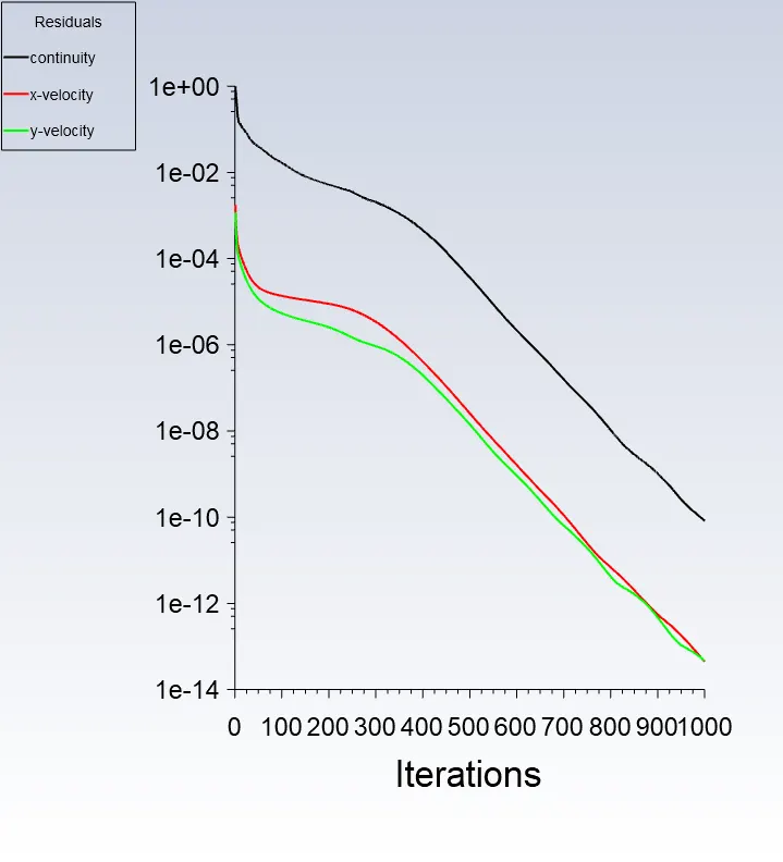
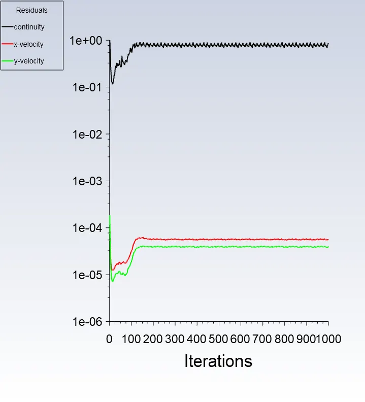
1. In both approaches, show that the flow has converged. That is, what quantities or plots need to be looked at to determine that the flow has converged?
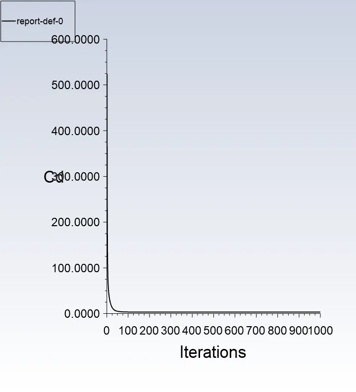
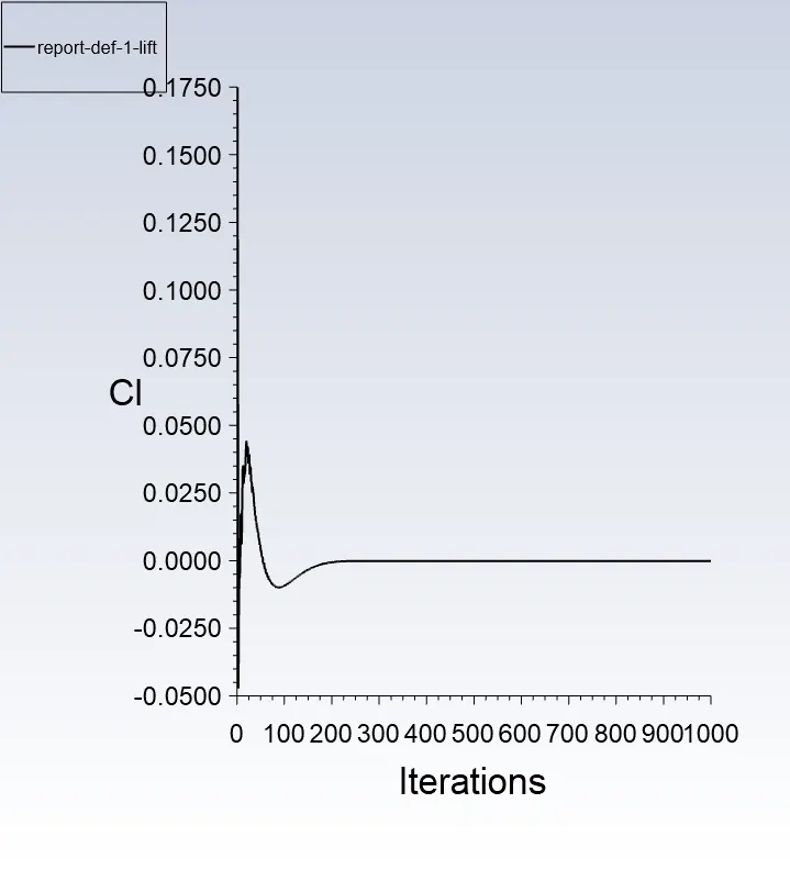
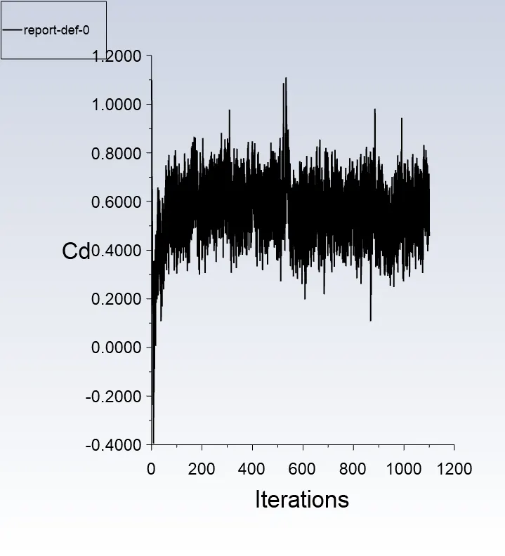
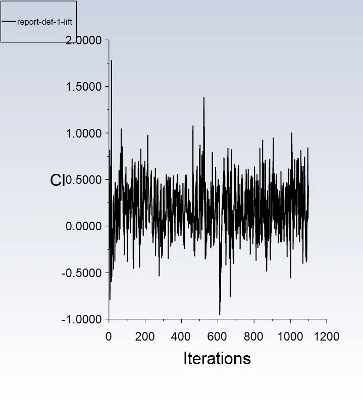
2. Plots of the coefficient of drag and lift.
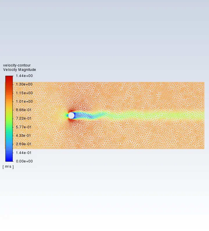
3. Plots to show vortex shedding behind the cylinder.
4. Mention the referred material (Reference Paper or Fluid Mechanics Textbook) at the end of the challenge submission page.

Theory :

Phenomenon of Karman vortex street :

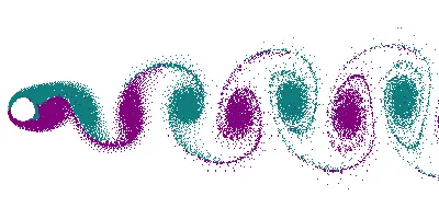
In fluid dynamics, a Karman vortex street is a repeating pattern of swirling vortices, caused by a process known as vortex shedding which is responsible for the unsteady separation of flow of a fluid around blunt bodies.

It is named after the engineer and fluid dynamicist Theodore von Karman and is responsible for such phenomena as the "singing" of suspended telephone or power lines and the vibration of a car antenna at certain speeds. Mathematical modeling of von Kármán vortex street can be performed using different techniques including but not limited to solving the full Navier-Stokes equations with k-epsilon, SST, k-omega and Reynolds stress, and large eddy simulation (LES) turbulence models, or by numerically solving some dynamic equations such as the Ginzburg-Landau equation.

Introduction :

Flow over a cylinder is one of the basic simulation in CFD domain and till this date the research is still going on to study the unsteady behaviour caused by the flow.The flow over cylinder study is very complex and periodic flow pattern are seen at lower Reynolds number and after achieving critical Reynolds number value, the flow get change in the wake region and this wake region can be studied using literature of Karman vortex street.one of the important point is Vortex shedding means In fluid dynamics vortex shedding is an oscillating flow that takes place when a fluid such as air or water flows past a bluff (as opposed to streamlined) body at certain velocities, depending on the size and shape of the body. In this flow, vortices are created at the back of the body and detach periodically from either side of the body forming a Von Karman vortex street. The fluid flow past the object creates alternating low-pressure vortices on the downstream side of the object. The object will tend to move toward the low-pressure zone.

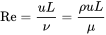
• Reynolds No. : The Reynolds number is the ratio of inertial forces to viscous forces within a fluid that is subjected to relative internal movement due to different fluid velocities. A region where these forces change behavior is known as a boundary layer, such as the bounding surface in the interior of a pipe. A similar effect is created by the introduction of a stream of high-velocity fluid into a low-velocity fluid, such as the hot gases emitted from a flame in air.

• With respect to laminar and turbulent flow regimes:
• laminar flow occurs at low Reynolds numbers, where viscous forces are dominant, and is characterized by smooth, constant fluid motion;
• turbulent flow occurs at high Reynolds numbers and is dominated by inertial forces, which tend to produce chaotic eddies, vortices and other flow instabilities.

  The Reynolds number is defined as

  

  where:

  • ρ is the density of the fluid (SI units: kg/m³)
  • u is the flow speed (m/s)
  • L is a characteristic linear dimension (m) (see the below sections of this article for examples)
  • μ is the dynamic viscosity of the fluid (Pa·s or N·s/m² or kg/(m·s))
  • ν is the kinematic viscosity of the fluid (m²/s).

• Strohaul No : It is a dimensionless number describing oscillating flow mechanisms. The parameter is named after Vincenc Strouhal, a Czech physicist who experimented in 1878 with wires experiencing vortex shedding and singing in the wind. The Strouhal number is an integral part of the fundamentals of fluid mechanics.

The Strouhal number is often given as

where f is the frequency of vortex shedding, L is the characteristic length (for example, hydraulic diameter or the airfoil thickness) and U is the flow velocity. In certain cases, like heaving (plunging) flight, this characteristic length is the amplitude of oscillation. This selection of characteristic length can be used to present a distinction between Strouhal number and reduced frequency:

where k is the reduced frequency, and A is amplitude of the heaving oscillation.

Drag Coefficient

In fluid dynamics, the drag coefficient (commonly denoted as: , or ) is a dimensionless quantity that is used to quantify the drag or resistance of an object in a fluid environment, such as air or water. It is used in the drag equation in which a lower drag coefficient indicates the object will have less aerodynamic or hydrodynamic drag. The drag coefficient is always associated with a particular surface area

The drag coefficient is defined as

where:

• is the drag force, which is by definition the force component in the direction of the flow velocity;
• is the mass density of the fluid;
• is the flow speed of the object relative to the fluid;
• is the reference area

Lift Coefficient

In fluid dynamics, the lift coefficient (C_L) is a dimensionless quantity that relates the lift generated by a lifting body to the fluid density around the body, the fluid velocity and an associated reference area. A lifting body is a foil or a complete foil-bearing body such as a fixed-wing aircraft. C_L is a function of the angle of the body to the flow, its Reynolds number and its Mach number. The section lift coefficient c_l refers to the dynamic lift characteristics of a two-dimensional foil section, with the reference area replaced by the foil chord

The lift coefficient C_L is defined by

,

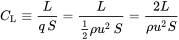where is the lift force, is the relevant surface area and is the fluid dynamic pressure, in turn linked to the fluid density , and to the flow speed .

Procedure :

Geometry Preparation :

For preparing our geometry, we will use spacelaim interface.

The first and foremost thing we need to check is our units.

We can perform this operation using File -> Space Claim Options -> Units -> Length -> Set it to Meters

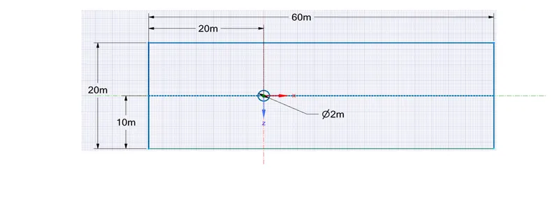
Here is our required geometry with dimensions specified.Now we to create a surface and delete the inner circle.

For that first of all we need to delete our construction lines. After that we need to convert our geometry as a surface using using 3d Mode Operation

We can perform this operation using Design -> 3D Mode -> Select the Geometry

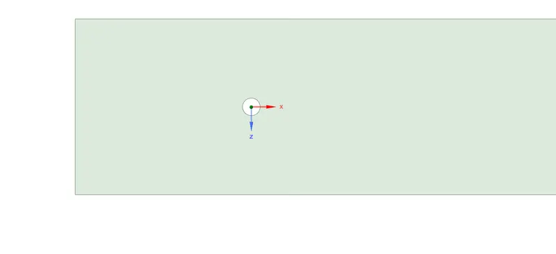
So, here is a glimpse of our final geometry.Now we can move to our next deck

Mesh Generation :

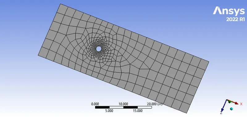
Here is a glimpse of the default mesh generated with the help of the default algorithm.

Here, first of all we need to fix the quads which are getting generated

We can perform this operation using Mesh -> Method -> Automatic Method -> Select the geometry -> Definitions -> Method -> Change it to Triangles -> Update Mesh

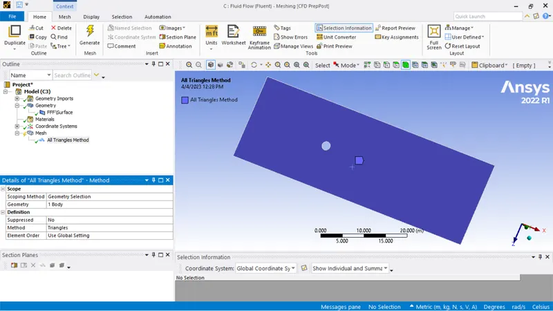
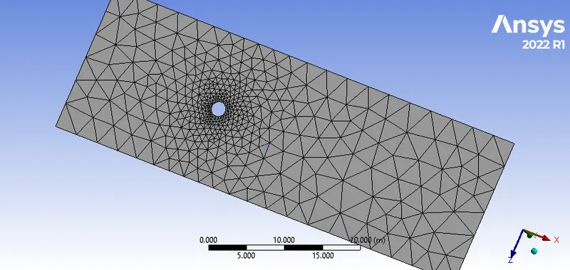
We can see the quads have been converted into triangles..Now we need to fine tune the default mesh generated

Now we to create Named Selection for our geometry

We can perform this operation using -> Edge Selection -> Select the edge -> Hit shorcut Key N -> Assign Names appropiately

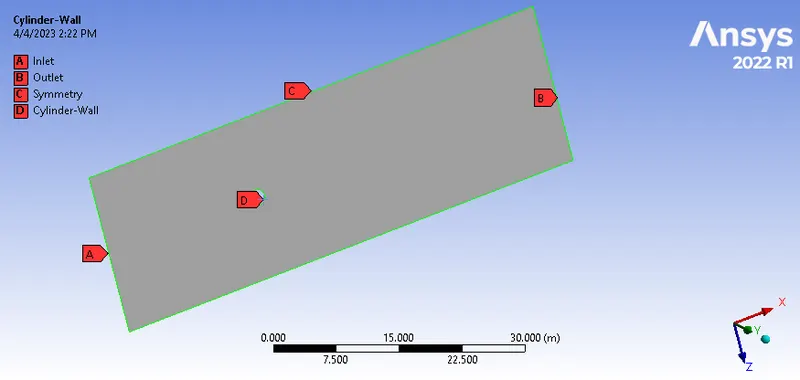
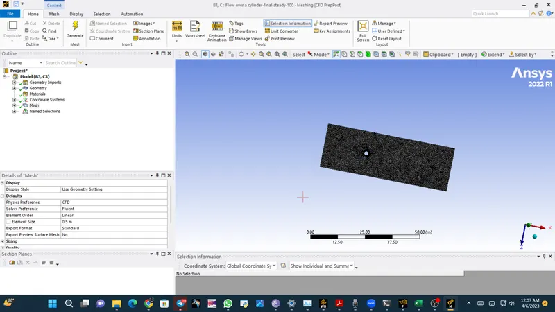
Now our next preference is the circular region, which look alike polygon..We need improve its edges using Edge Sizing Method

We can perform this operation using Mesh -> Insert -> Sizing -> Select the edges -> Definition -> Type -> No. Of Edges ( i.e 360/10 = 36 edges) -> Update It.

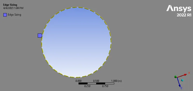
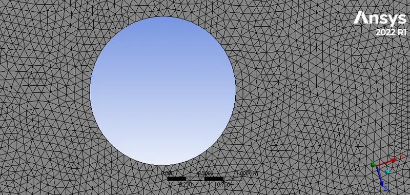
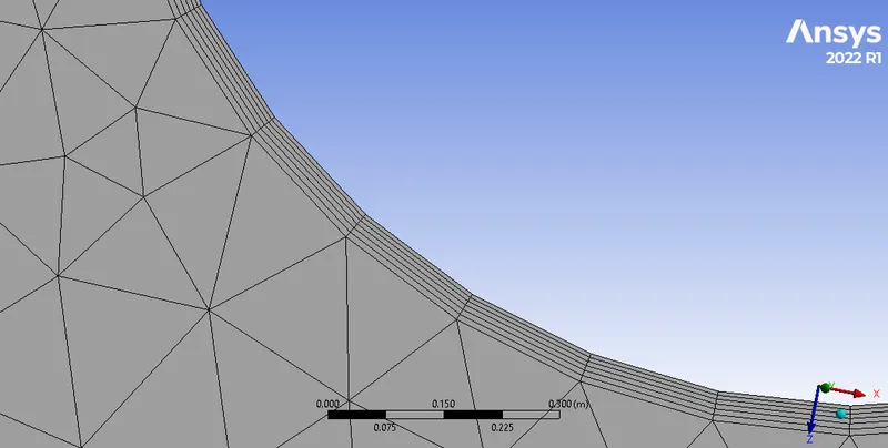
Now to fine tune edges near circular region we need to add Inflation Layers

We can perform this operation using Mesh -> Inflation -> Geometry Selection -> Select the whole geometry -> Boundary -> Select the edge -> Inflation Options -> First Layer Thickness -> First layer height -> 5.0e-3 meters -> Inflation Layers -> 6 -> Growth Rate -> 1.1 -> Update mesh

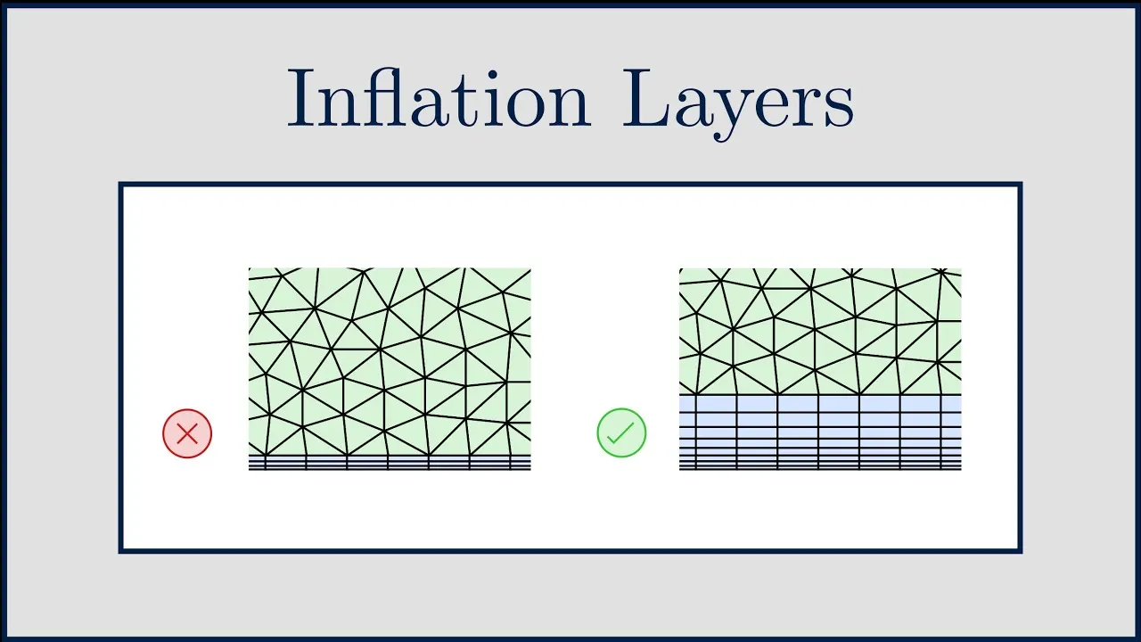
Inflation Layers

The inflation layer control is designed to create thin elements that can capture the normal gradient with minimal elements; use inflation layers to correctly capture the velocity and temperature gradients near no-slip walls.

Inflation is related to meshing. The finer our mesh is, the more accurate our results are. However, if the mesh is finer throughout the domain, it will require more computation time for the solvers. So we fine-mesh only where there is a great variation in results, or in the area where we are interested in seeing the nature of flow, for example. Near the wall, the boundary layer is formed as the velocity changes; in order to obtain these results, we need a very fine mesh near the wall. Hence, we create inflation by selecting the wall boundary and number of layers in Ansys. Inflation is nothing but creating a fine mesh or layers of fine mesh on the area of interest in the domain.

Setup :

Solving Steps :

Case 1 Simulate the flow with the steady case and calculate the Strouhal Number for Re= 100.

• Domain -> Mesh -> Check Mesh Quality
• Setting Up Physics
• Solver Type -> Pressure Based -> Velocity -> Absolute -> Time -> Steady
• Viscous Nature -> Laminar
• Material Selection -> User-Defined-Air with density of 1 kg/m^3 and viscosity of 0.02 kg/ms

`Re=(ρ V D)/μ`

Re = 100

ρ = 1 kg/m^3

V = 1 m/s

D = 0.2 m

`µ = (1×1×2)/100 = 0.02`

After Putting it into Reyonlds Equation, Viscosity comes out to be 0.02 kg/ms

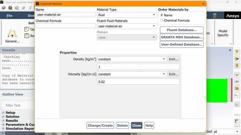
• Cell Zone -> Replace the default air with our user defined air material and now we can delete the default air from our Material Selection Tab

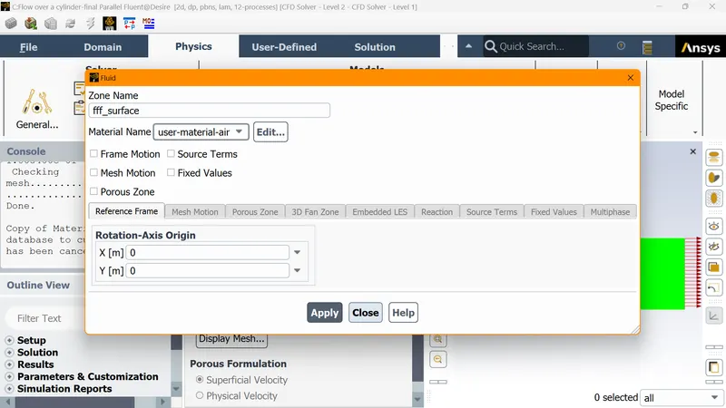
Boundary Condition

• Inlet -> Velocity Inlet -> Velocity 1m/s
• Outlet -> Pressure Outlet -> Gauge Pressure
• Cylinder Wall -> Wall -> Stationary -> Shear Condition -> No Slip

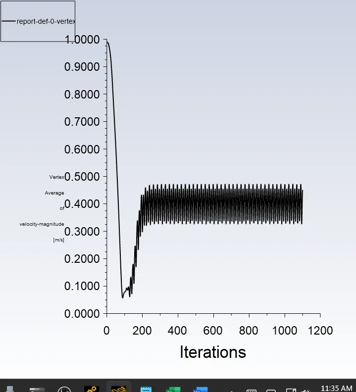
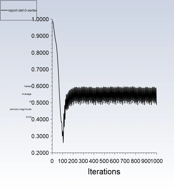
Now, we need to create a monitor point for monitoring our velocity flow

We can perform this operation using Results -> Create -> Monitor Point -> Distance of 4D at the right side of cylinder.

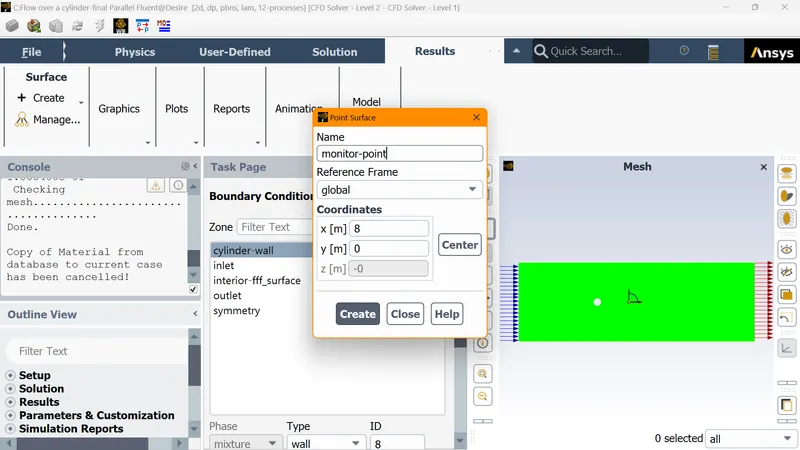
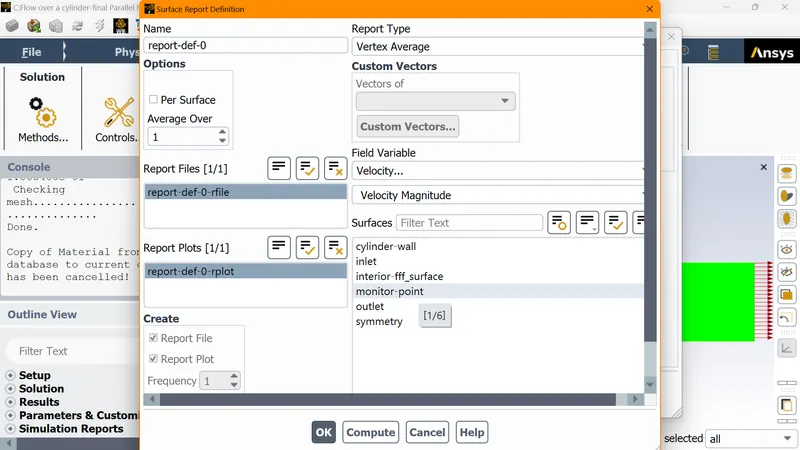
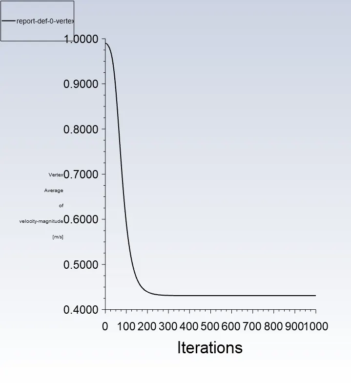
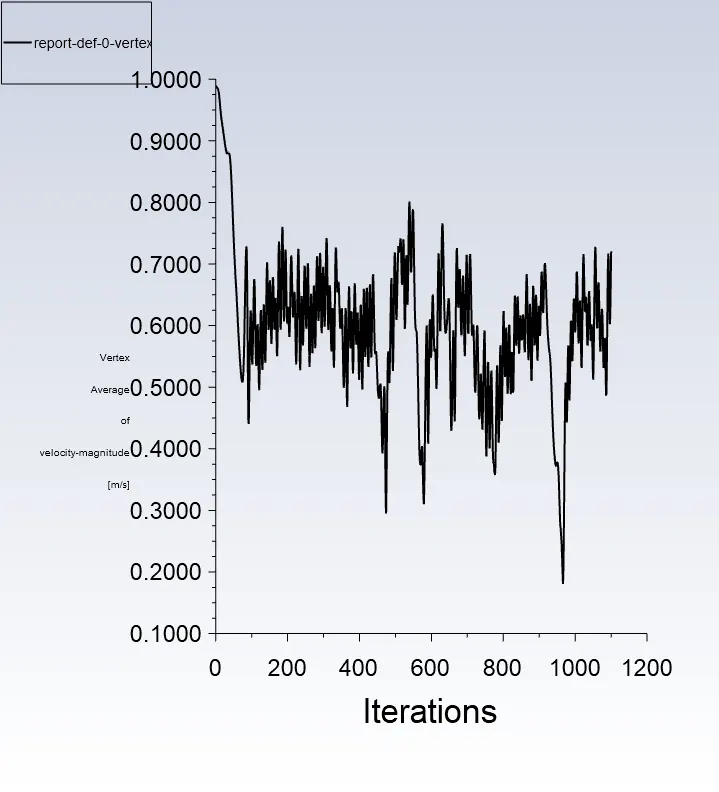
• Report Definitions -> New -> Surface Report -> Vertex Average -> Field Variable -> Velocity -> Surface -> Monitor-Point

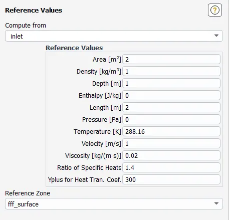
• Reference Values -> Compute from -> Inlet -> Frontal Area -> 2 m^2 -> Length -> 2 m

• Initilization -> Hybrid Initilization -> Run
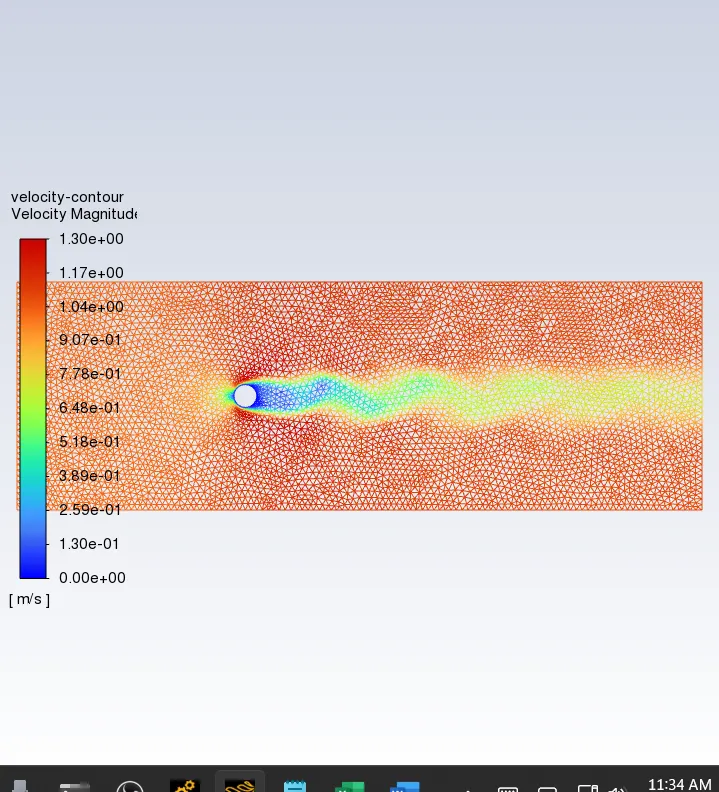
• Contour -> New -> Velocity Contour > Compute

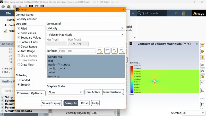
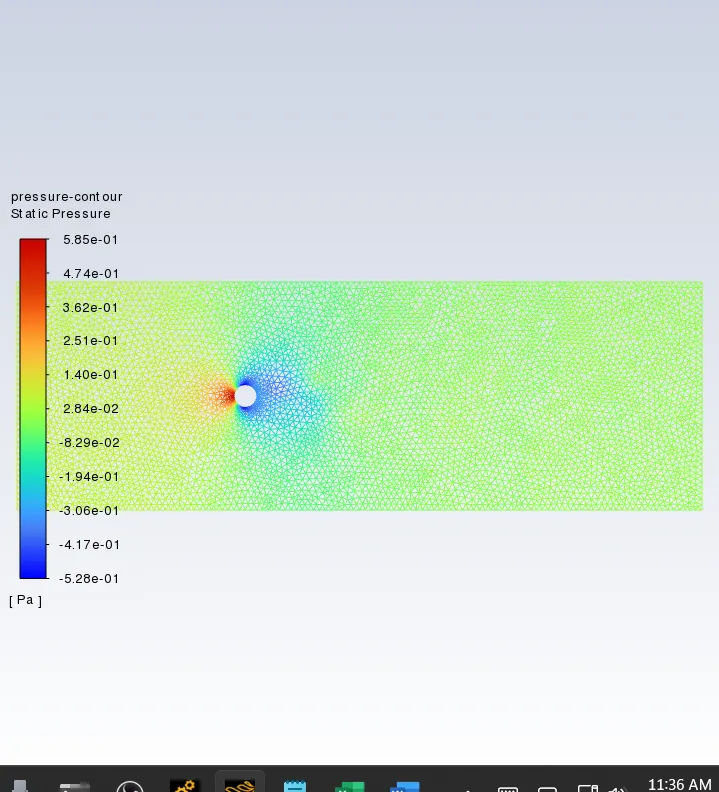
Similarly Pressure Contour is also computed

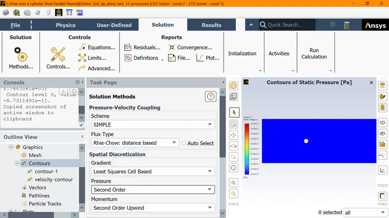
• Solution Methods

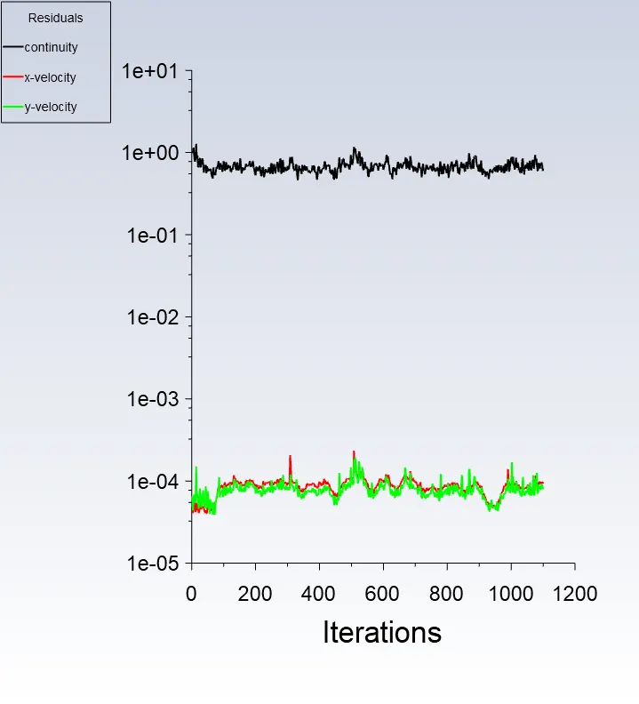
• Residuals

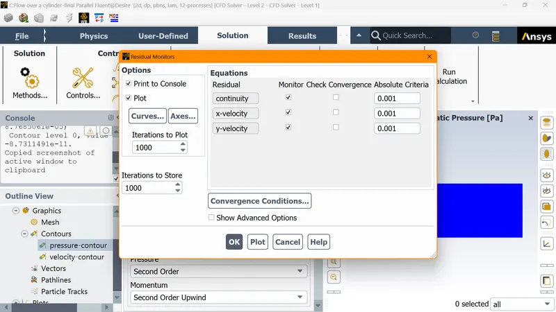
Here, we want to see the plots until our iterations are over, not until the solution gets converged.

Now we need to visualize Velocity Animations also

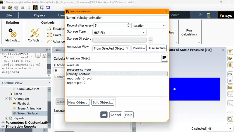
Results

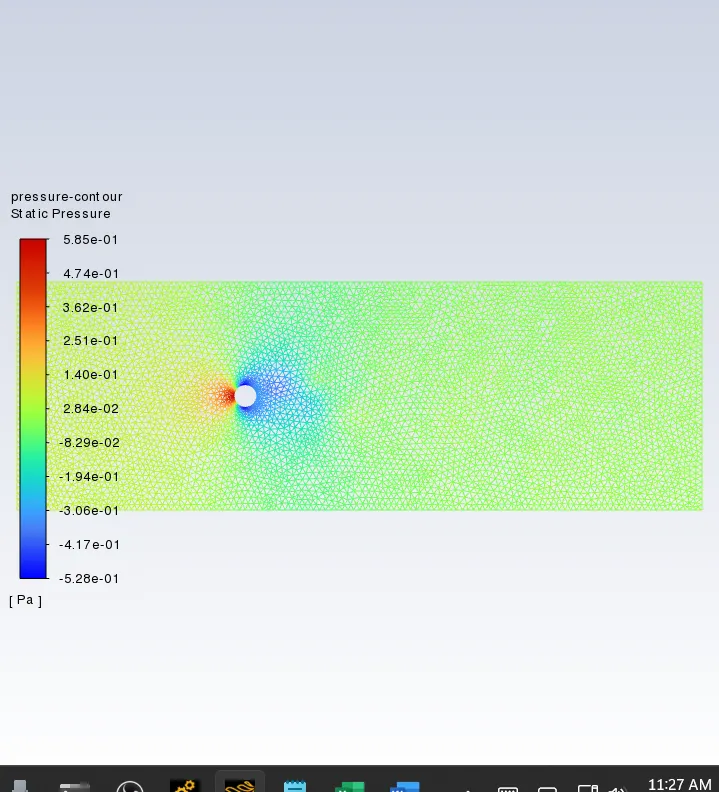
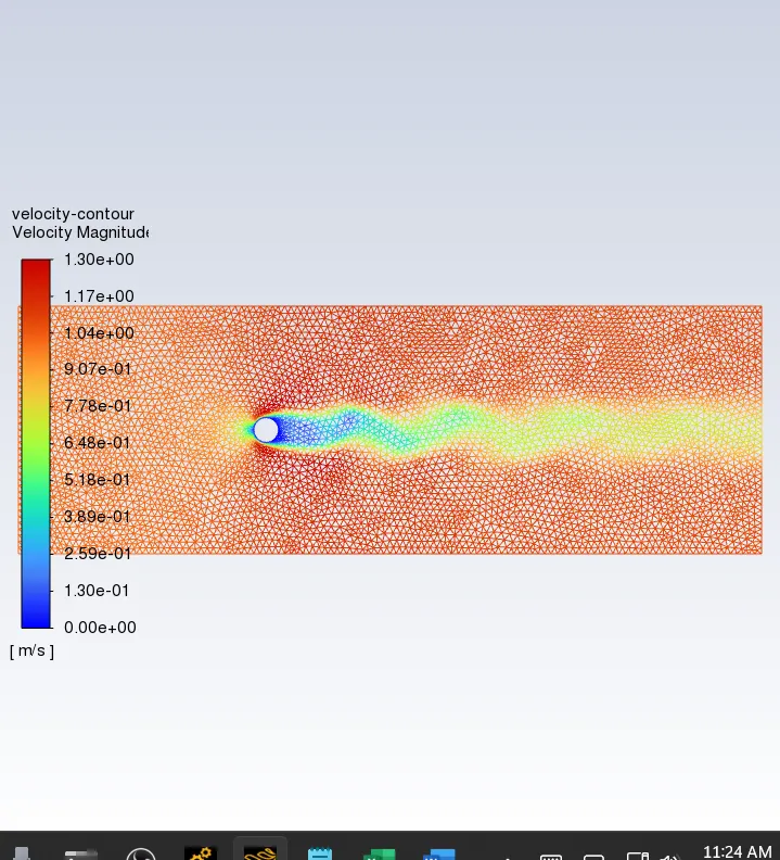
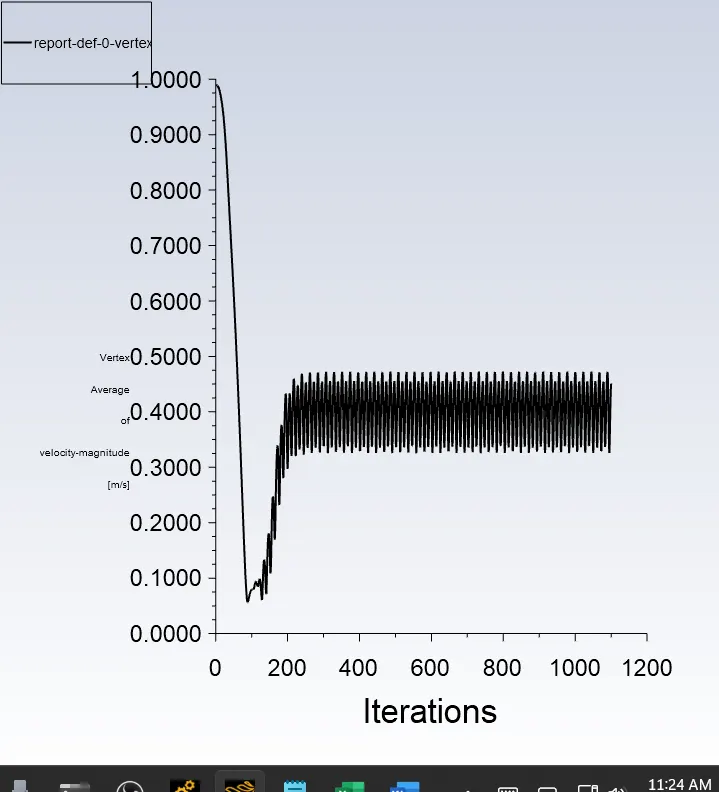
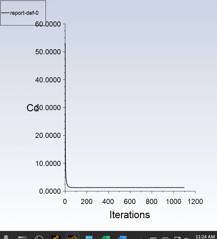
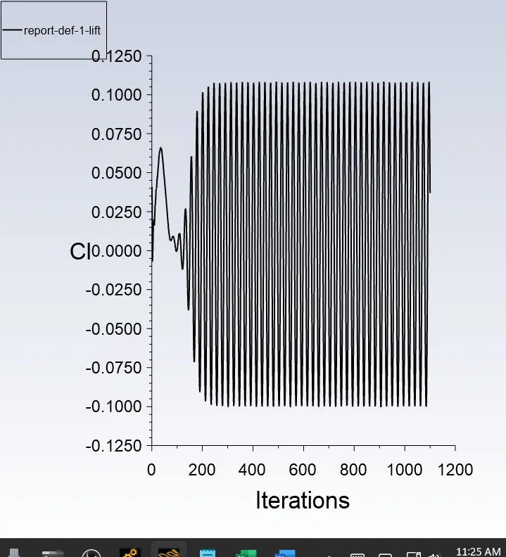
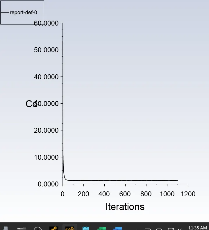
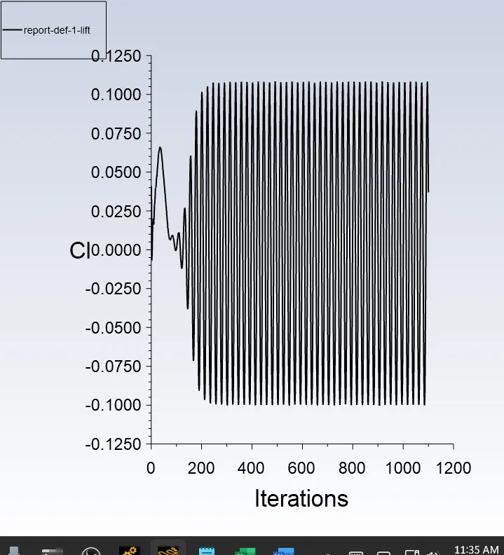
Here are the results in steady state over 1100 iterations..Here we can observe that the values of Lift Coefficient is almost constant and we can conclude that the flow has converged.

Reynolds Number	Viscosity	Lift Coefficient	Drag Coefficient	Vertex Average at monitor point(m/s)
100	0.02	0.03694372	1.3197326	0.45109755

Case 1: Simulate the flow with the unsteady case and calculate the Strouhal Number for Re= 100.

Setup :

Solving Steps :

• Time -> Transient State
• Initilization -> Hybrid Initilization
• Time Step Size -> 0.1

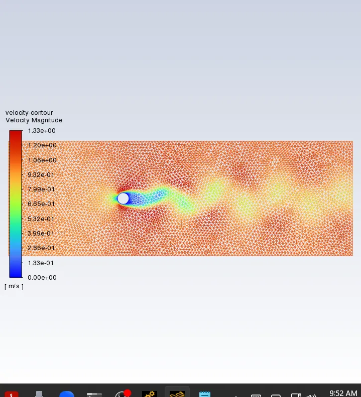
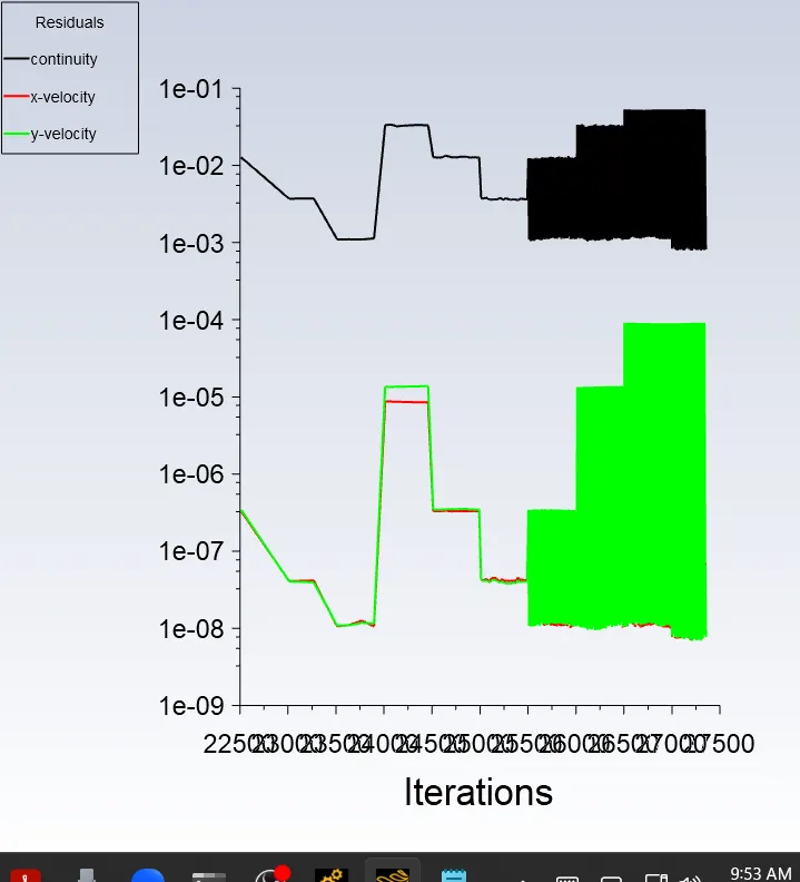
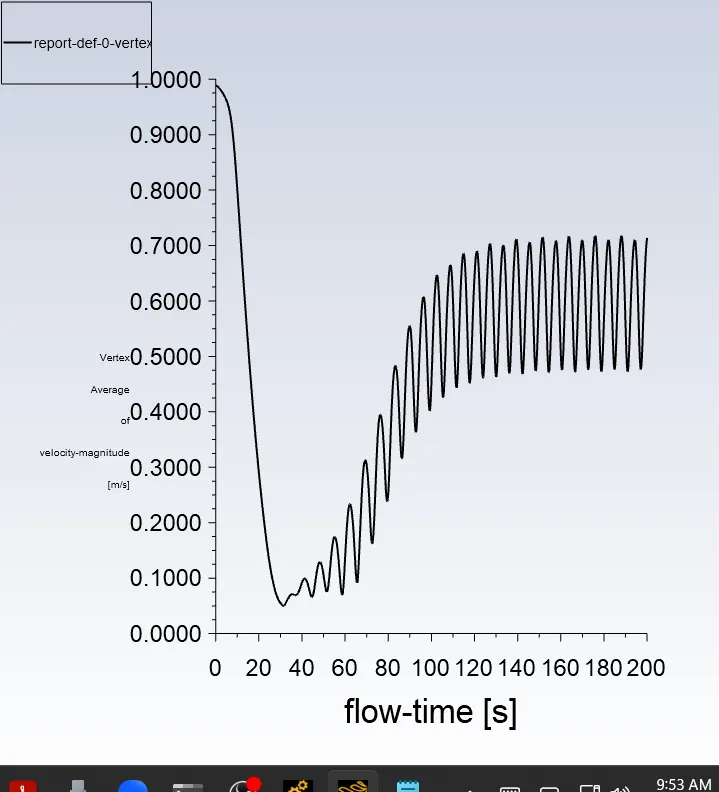
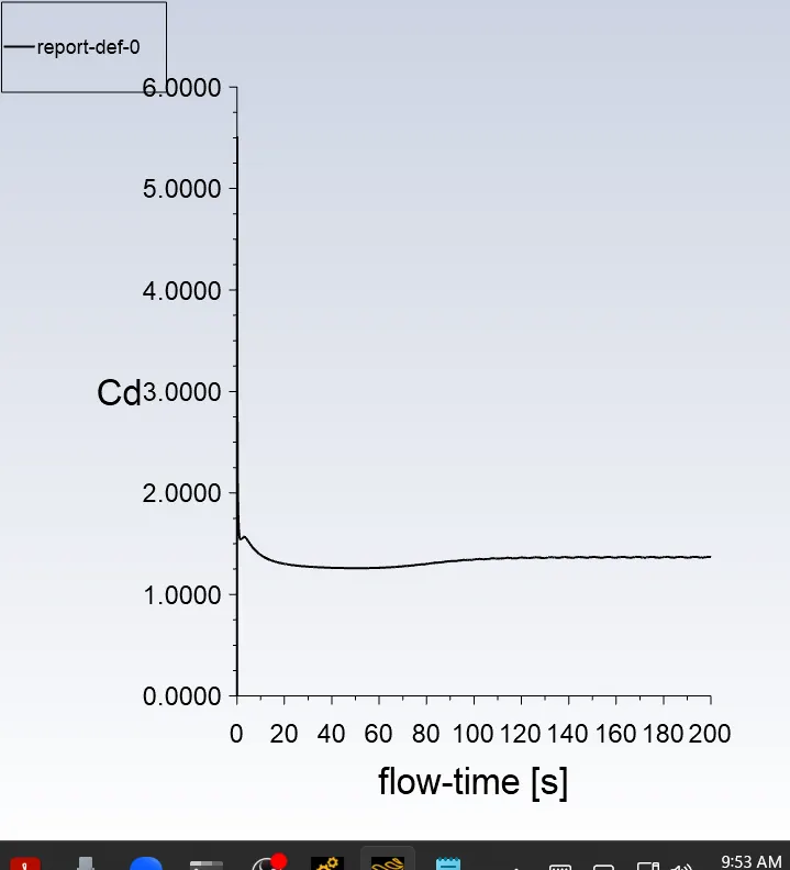
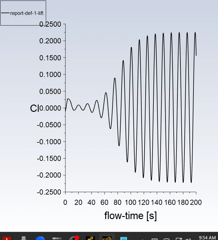
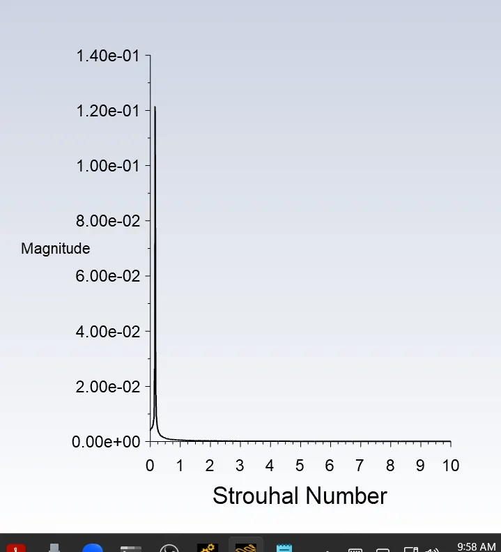
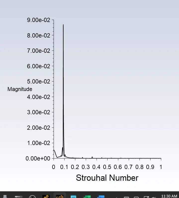
Reynolds Number	Viscosity	Strohaul Number	Frequency of Vortex Shedding	Lift Coefficient	Drag Coefficient	Vertex Average at monitor point
100	0.02	0.26	0.13	0.15553168	1.3703797	0.7138558

St = (No of Peaks)/(Flow Time)×(Characteristics Length)/Velocity

No of Peaks = 26

Flow time = 200

Characteristics Length = 2 m

Velocity = 1 m/s

Strohaul Number = 0.26

Case 2 :

For Reynolds No 10 -> Viscosity -> 0.2

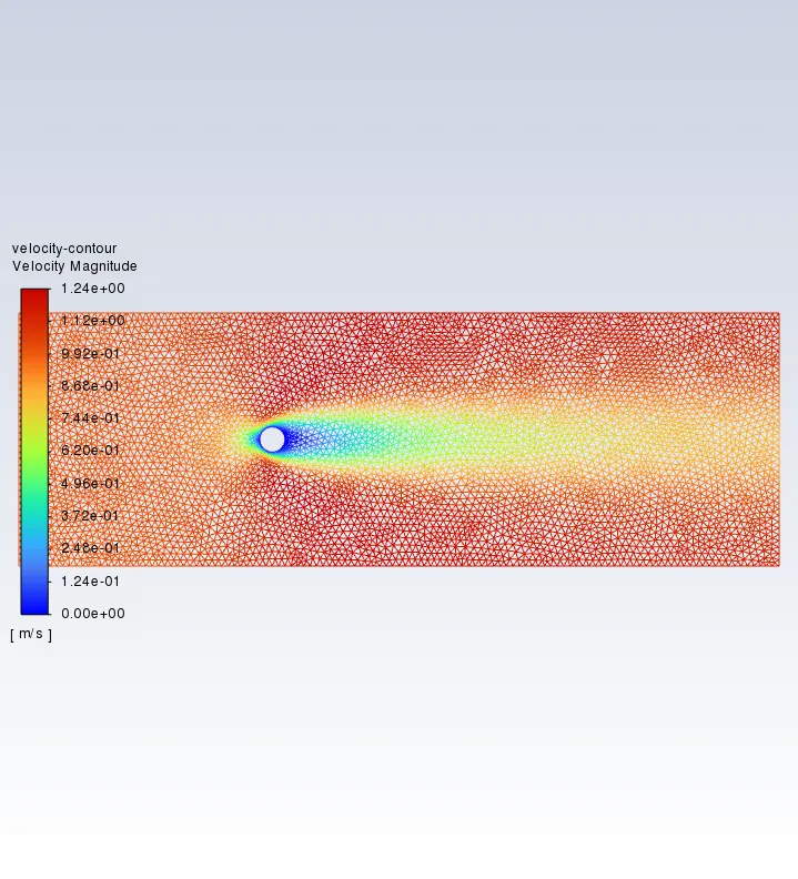
For Reynolds No 100 -> Viscosity -> 0.02

For Reynolds No 1000 -> Viscosity -> 0.002

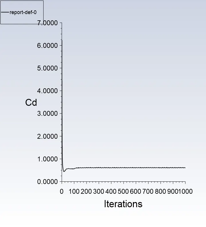
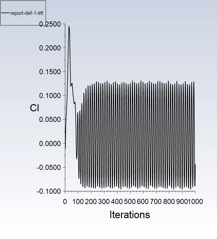
For Reynolds No 10000 -> Viscosity -> 0.0002

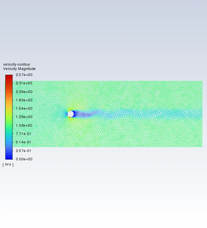
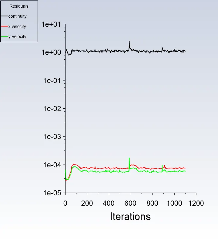
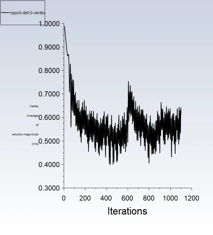
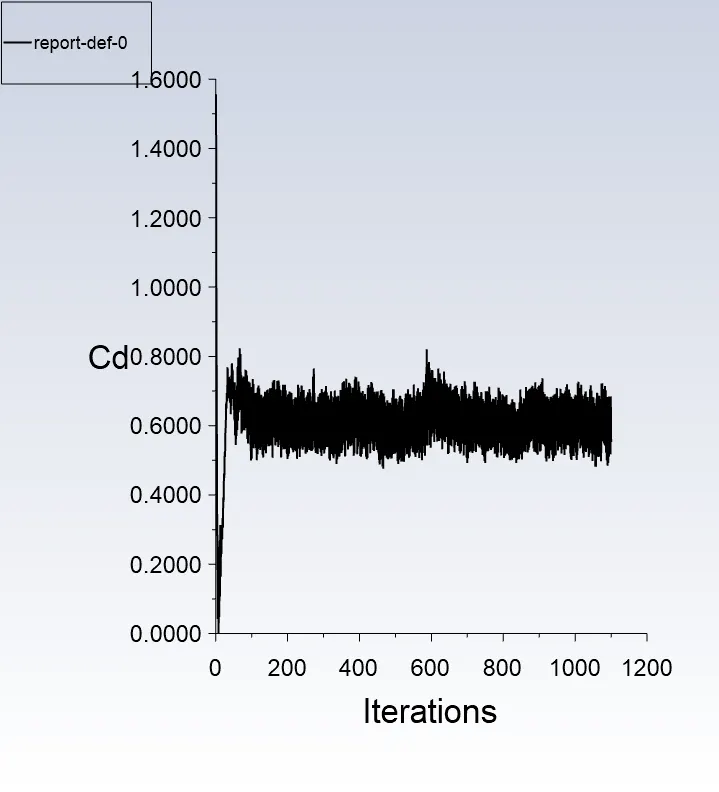
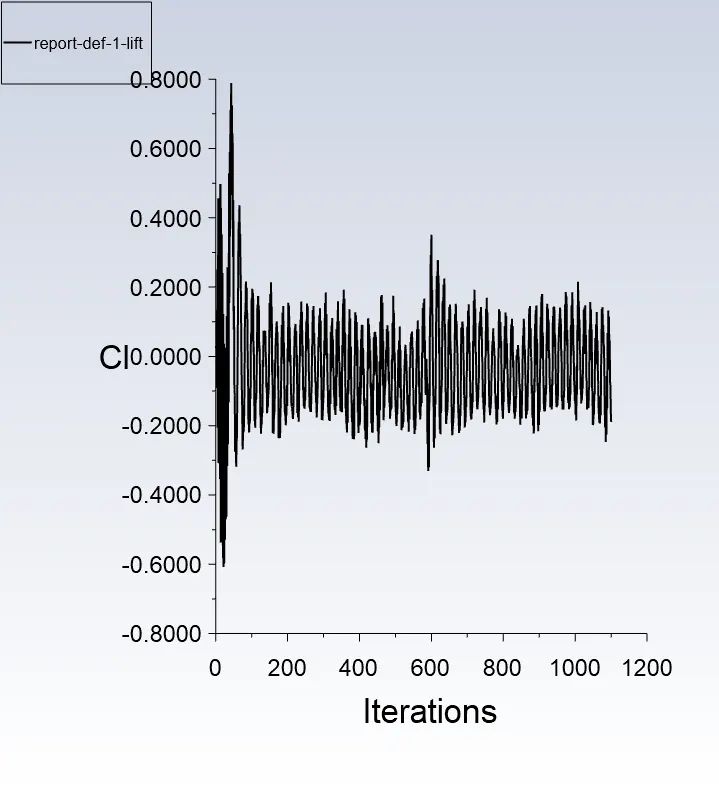
For Reynolds No 100000 -> Viscosity -> 0.00002

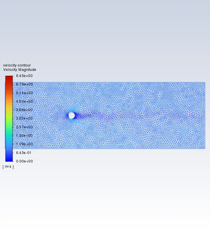
Results Comparision

Reynolds Number	Viscosity	Lift Coefficient	Drag Coefficient
10	0.2	-0.00017861751	3.3138534
100	0.02	0.03694372	1.3197326
1000	0.002	-0.043762027	0.60394287
10000	2.0E-4	-0.18957602	0.55303212
100000	2.0E-5	0.43651073	0.45885699

Conclusion :

1. From the above Result Comparison Table, we can conclude that Reynolds Number and the Drag Coefficient are inversibly proportional in nature with respect to each other, as we can observe that the Drag Coefficient value is constantly decreasing with an increase in Reynolds Number.

2. For Reynolds No = 100 and unsteady case, Strohaul Number value came out to be 0.26 & Drag Coefficient value came out to be 1.3703797

3. From the results, we can conclude that a refined mesh is desired for perfect results, but on the contrary, it will increase computational time drastically.

References

• Fluid Mechanics Frank M White

Video Animations

Vortex Shedding Phenomena with Reynolds No 100 and mesh size 0.1 m

Vortex Shedding Phenomena with Reynolds No 100 and mesh size 0.5 m