Week 2 - Flow over a Cylinder.
Steady and Unsteady flow Past Cylinder
Aim: To simulate the steady and unsteady flow over cylinder and Validate results
For given Ryenolds number 10 ,100,1000,10000,100000
and calculate Struohal number for Re=100 and
drag and lift coff for all other renoulds number
INTRODUCTION & THEORY
Phenomenon of Karman vortex street
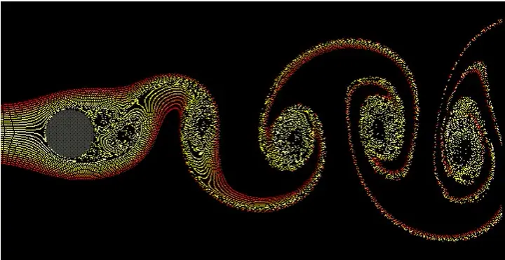
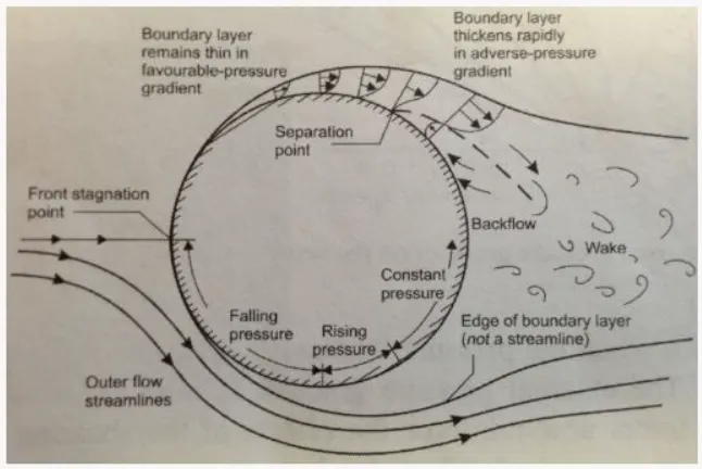
Physics behind vortex formation :
'It occurs when a fluid flows around a cylindrical object. The pressure on a fluid particle rises to the stagnation pressure as it hits the leading edge of the object. As it trails along the boundary layer of the rounded surfaces (one on each side of the cylindrical object), the high pressure is not sufficient enough to force the flow about the back of the cylinder. Therefore the, near the widest section of the cylinder, the boundary layers separate from the surface of each side of the object and form two shear layers that flow into the wake. The slower of the shear layers, flows closest to the object. This is when the vortex start to occur. As this slower shear layer rolls into the wake before the faster layer, they fold on each other and form swirling vortices'.
The bolded part is specifically what I don't understand. High pressure isn't sufficient enough to force the flow about the back of the cylinder? What does this mean? I would assume that it IS the pressure that forces the flow down and into the start of a vortex.
Geometry : -
2D geometry - showing the flow is passing across a vertical cylender is design in spaceclaim software. Geeneral concideration for fluid control volume is
frontal length - cylender dia(characterstics length ) * 10
Rear length - cylender dia(characterstics length )* 20
Width - cylender dia(characterstics length )*10
this can be achive by using some tools like construction lines, circles, rectangles.
The diamention of fluid domain and cylender is shown below.
Final geometry is shown below. To design right physics the inside circuler surface is to be deleted to carry out the simulation. Converting the geometry into the surface by using command pull and select.
Meshing:-
- Now in the mesh mode we set the mesh size, edge sizing and give inflation layers to the cylinder.
- The mesh size given is 0.25m (Method: Initially, Ansys meshing creates a quadrilateral dominant mesh. We need to convert it into Triangles.
- Go to Mesh
- →
- Insert
- →
- Method
- →
- Select face
- →
- Method(Triangles)
- →
- Generate Mesh
- Go to Mesh→ Insert → Method → Select face → Method(Triangles) →Generate Mesh
- ),
- edge sizing 4 (Sizing: The cylinder we have is not perfectly circular, so if we proceed like that geometry there might be inaccuracy in results. This option will help us to create smooth curves by dividing the circle into large numbers of edges.
- Go to Sizing
- →
- Select Edge
- →
- Type (Number of divisions)
- →
- Enter number and Generate Mesh
- Go to Sizing→ Select Edge→ Type (Number of divisions)→ Enter number and Generate Mesh
- ) after edge sizing image is shown below.
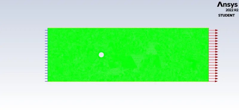
And the obtained mesh is shown below -
- 10 layers inflation layers with first layer thickness and first layer height of 0.005(Inflation: In order to resolve boundary over the cylinder we will require finner mesh around the cylinder. This option will let us create a finner 'body-fitted mesh' as the flow around the cylinder is quite important.)
Mesh Quality : -
The above graph shows better mesh quality and can obtain mesh independent output which can be used for the simulation.
Part Name :-
To set the desired boundaries and to give boundary conditions part naming is to be done after creating the mesh into to the Ansys mesher.
As Shown in above image we can see that as goemetry is symmetric thus symmetry B.C. is used and for cylender no slip wall is used. The naming done according to boundary conditions.
Fluent Setup:
First run Perform Check mesh in order to find any kind of errors in the geometry.
In this simulation we need to perform a vortex shedding formed by flow over a cylender thus we need to set physics according to flow. In vortex sheeding the important parameters are fluid material density and viscocity. This new material is doveloped in the fluent database.
General:
Solver- Pressure Based.
Velocity formulation- Absolute.
Time- Based on the case study we are going to do (Steady/Unsteady).
2D Space- Planer
Model:
Viscous model- Laminar
Materials:
Create/Edit- User_defined_fluid (The fluid is created such that only viscosity will be resopnsible for varing Reynold's number.)
Name- User_defined_fluid
Properties- Density (kg/m3)= 1 (constant)
Viscosity (kg/m-s)= 0.05 (constant)
To check the vortex nature it is important to know the Reynolds no.
Reynolds No.
The Reynolds number is a measure of the ratio of inertial to viscous forces in the flow of a fluid and may be defined as:
Re = ρVD/ μ
where:
ρ = Density,
D = the diameter of the cylinder around which the fluid is flowing,
V = the steady velocity of the flow upstream of the cylinder and
μ = the kinematic viscosity of the fluid.
Using Reynolds no. , viscocity of fluid, density of fluid and cylender dia we can find out the velocity magnitude of flow as mention in above Reynolds No. theory
Boundary Conditions:
Inlet- Velocity Inlet
Velocity Magnitude- for Re = 10--->0.25 m/s
for Re = 100--->2.5 m/s
for Re = 1000--->25 m/s
for Re = 10000--->250 m/s
for Re = 100000--->2500m/s
Outlet- Pressure outlet
Gauge Pressure- 0 Pa
Symmetry- Symmetry
Zone name- Symmetry
Walls- Wall
Wall motion- Stationary wall
Shear condition- No slip
Report Definations
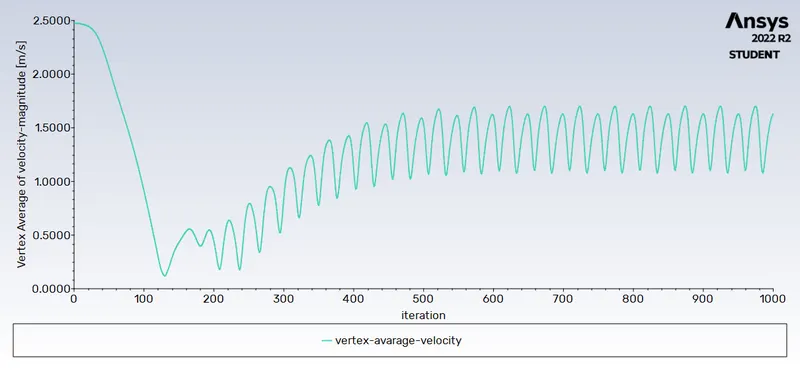
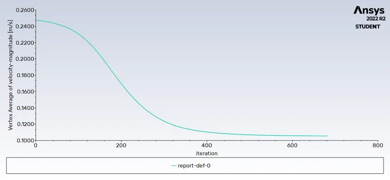
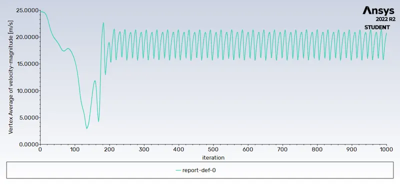
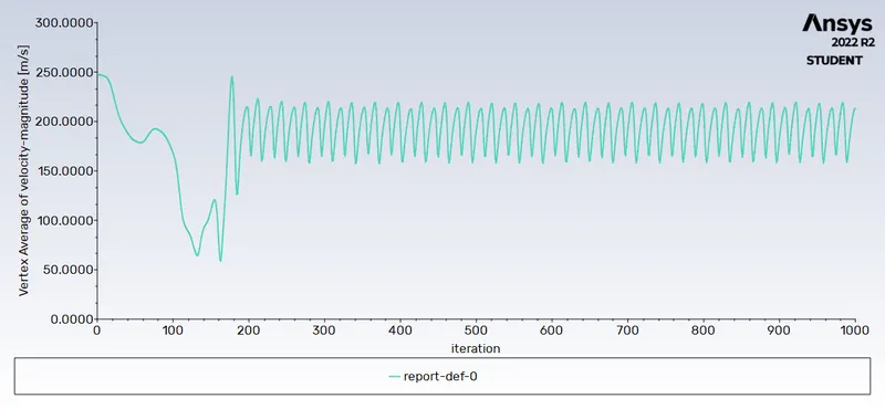
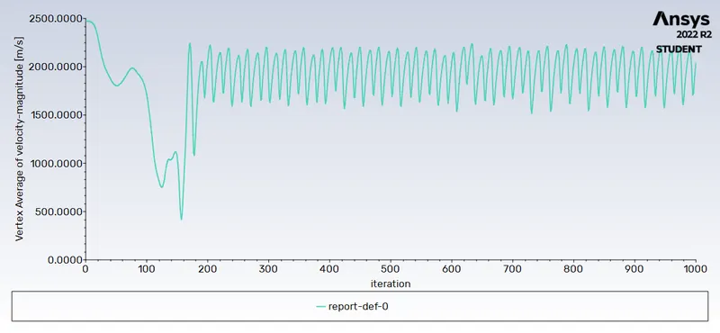
Create a Vertex average of velocity magnitude using surface report at a monitor point 8m away from the center of the cylinder to the right of the cylinder along X-direction.
to read a average velocity value at above monitor point go to definations - surface report - vertex average.
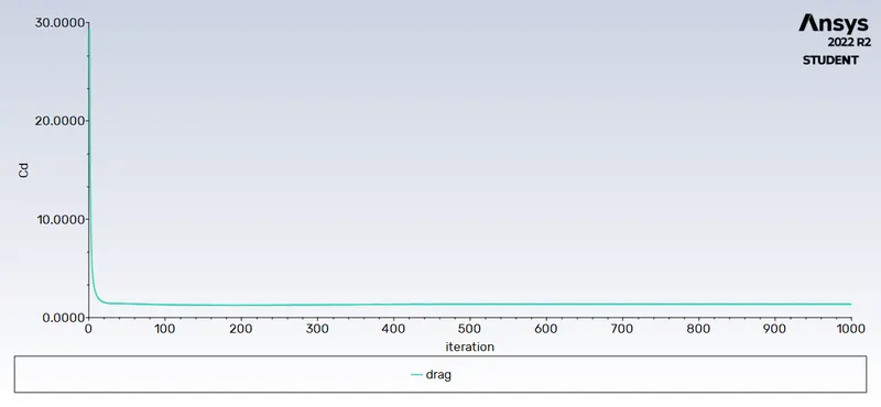
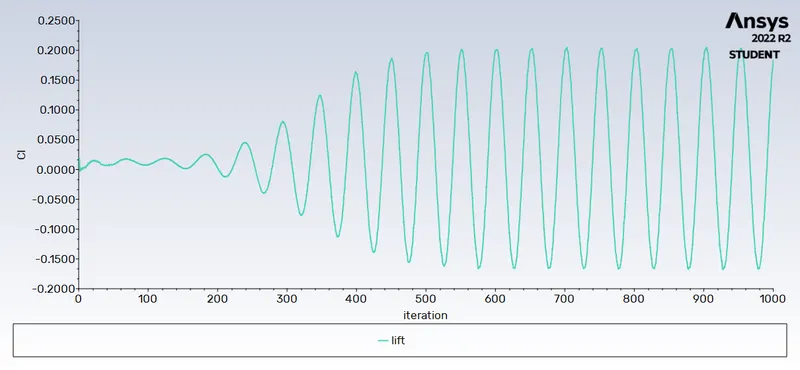
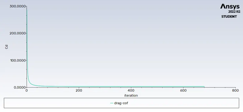
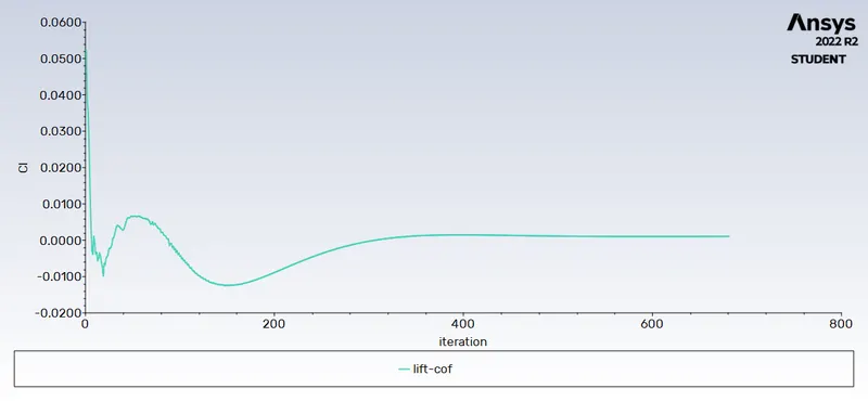
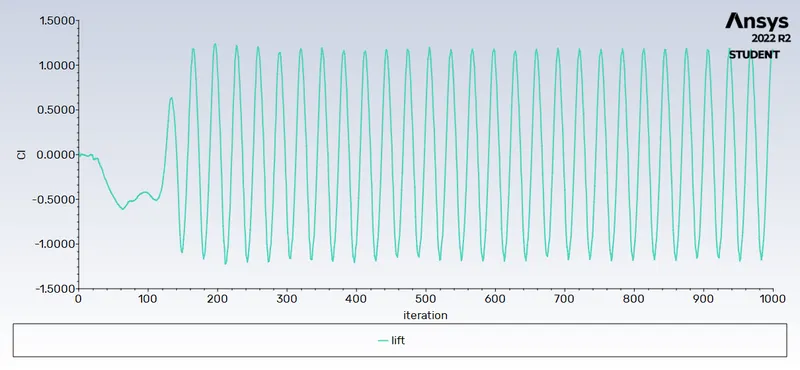
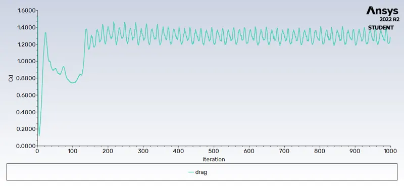
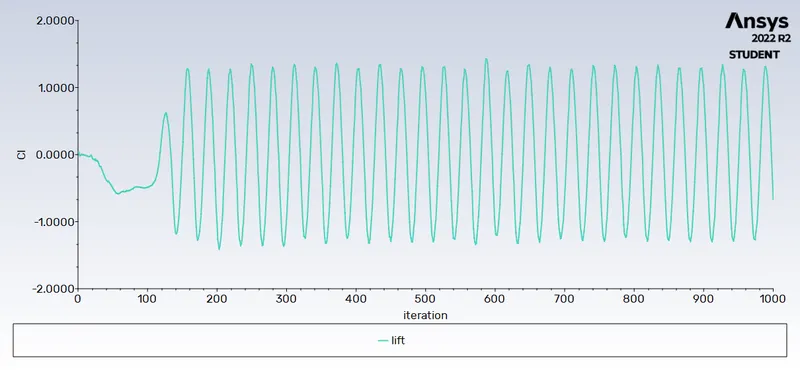
Coefficient of Drag and Coefficient of Lift report created using force report.
For drag go to definations - new - force report - Drag
For lift go to definations - new - force report - Lift
Plots :-
In both i.e. steady and unsteady state simulations, following plots are to be shown:
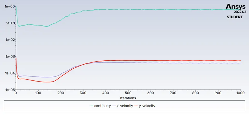
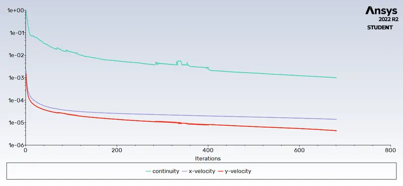
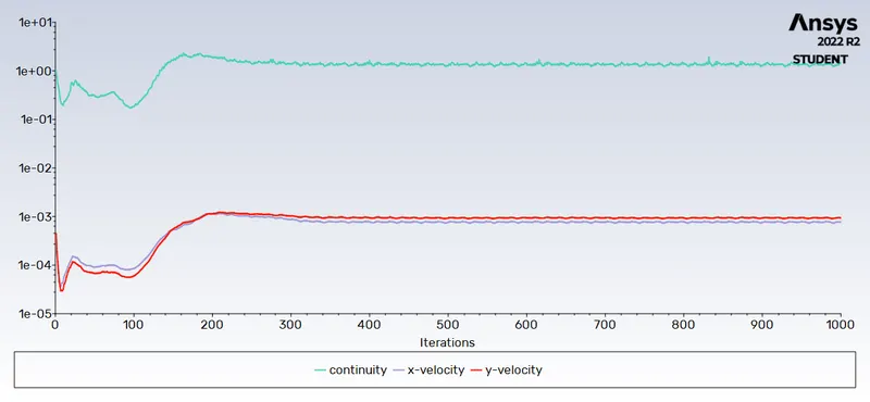
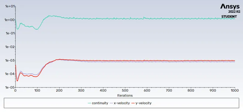
- Residual plot - This plot helps us in knowing at what point convergence is achieved.
- Monitor point velocity plot - A monitor point is placed at a distance of 8m from the cylinder in order to calclate the velocity at that point.
- Drag coefficient plot - To calculate the drag coefficient.
- Lift coefficient plot - To calculate the lift coefficient.
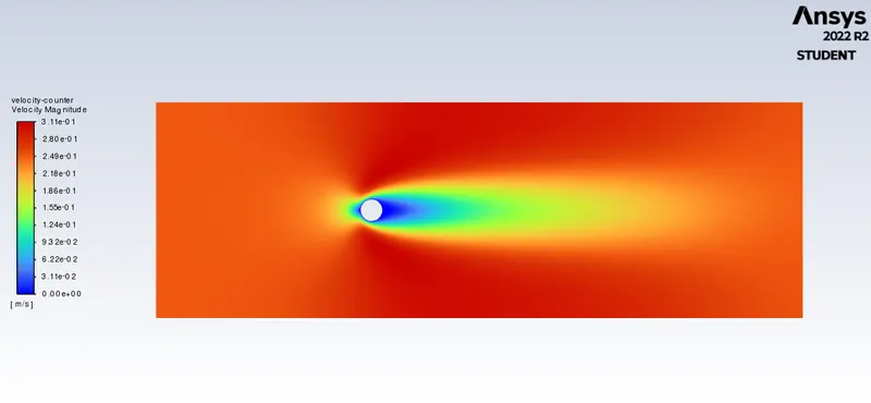
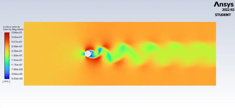
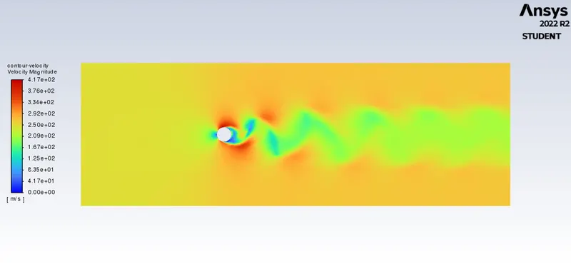
- Velocity contour plot - To see the velocity changes in the flow over the cylinder.
Initialization method- Hybrid for STEADY STATE simulations
Standard for UNSTEADY STATE simulations
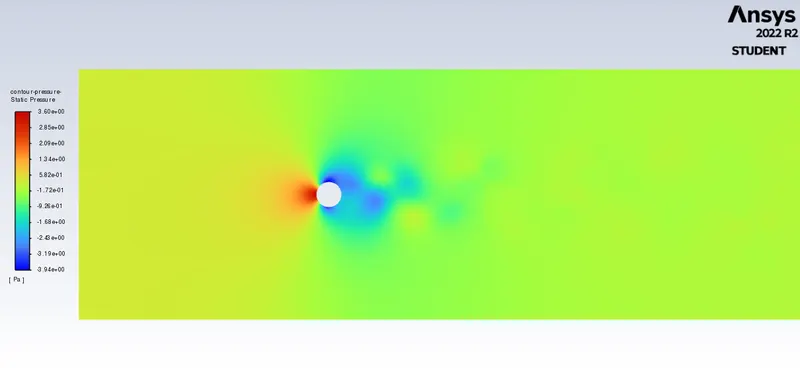
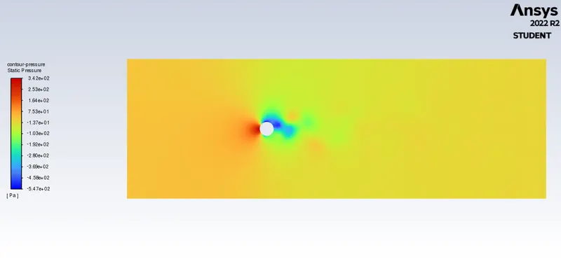
- Contour plots of Pressure & Velocity - Shows the velocity and pressure distribution.
Reference Values was set to:
Area-2 Sq.m
Length-2 m;
Depth-1m;
Density-1 kg/m
Velocity-2.5 m/s;
Dynamic Viscocity- 0.02 kg/m-s;
PART 1
Steady state Re=100
V=2.5m/s
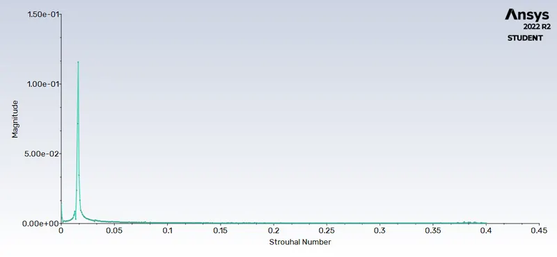
Strouhal Number [3]:
The Strouhal Number is a dimensionless value useful for analyzing oscillating unsteady fluid flow dynamics problems.
Strouhal number cannot be calculated for the steady state as there is no time parameter which is required in frequency calculation and can only be calculated for unsteady state condition.
The Strouhal Number can be expressed as
St=ω⋅Lv">St=ω⋅LvSt=ω⋅Lv
where St = Strouhal Number
ω">ωω= oscillation frequency
L = characteristic frequency
v = flow velocity
The Strouhal Number can be important when analyzing unsteady, oscillating flow problems. The Strouhal Number represents a measure of the ratio of the inertial forces due to the unsteadiness of the flow or local acceleration to the inertial forces due to changes in velocity from one point to an other in the flow field.
ω=">ω=ω=No.of peaks/Flow time
St=1.00e-1
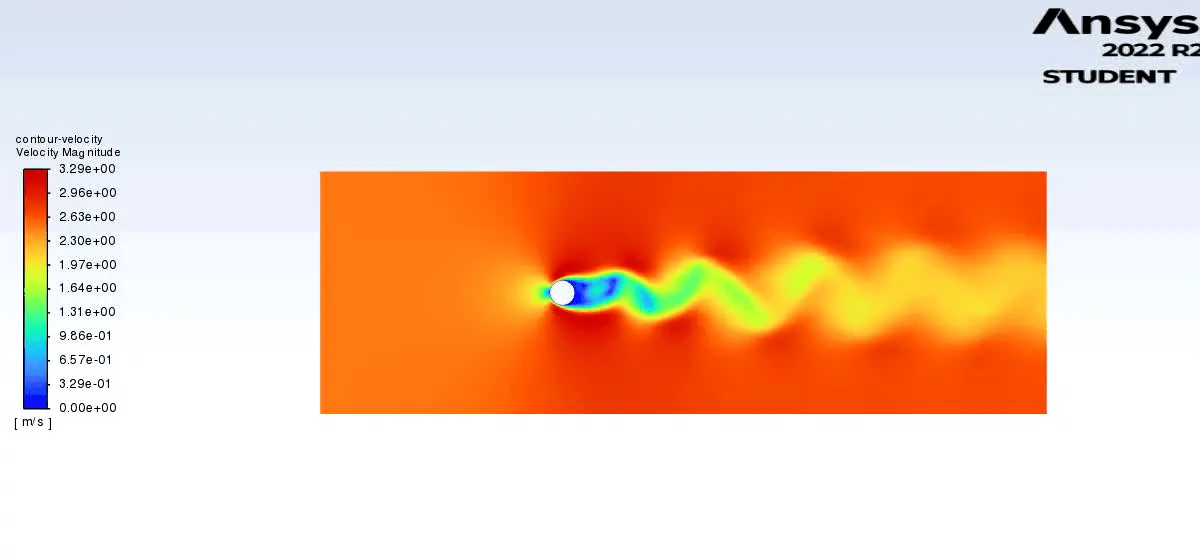
Unsteady state
Re=100
v=2.5m/s
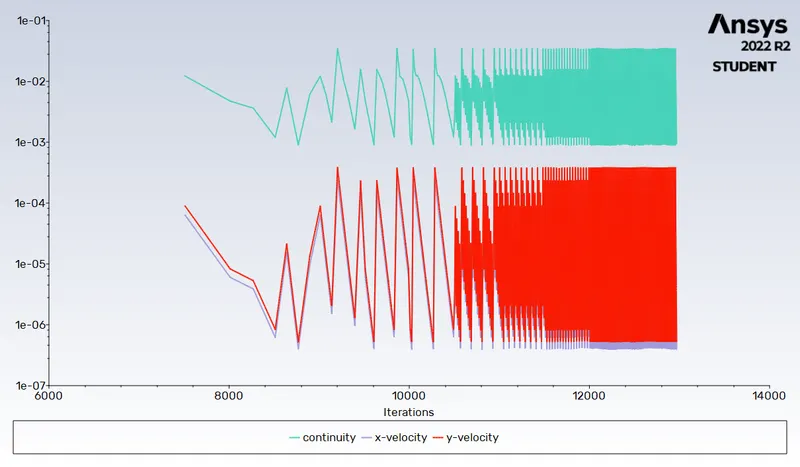
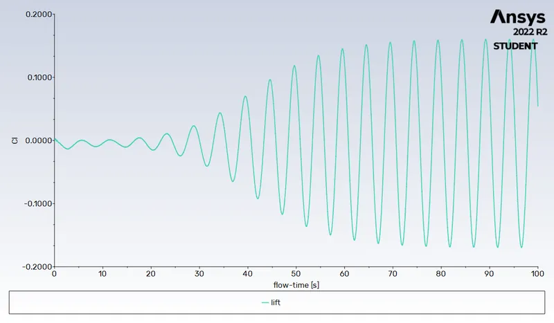
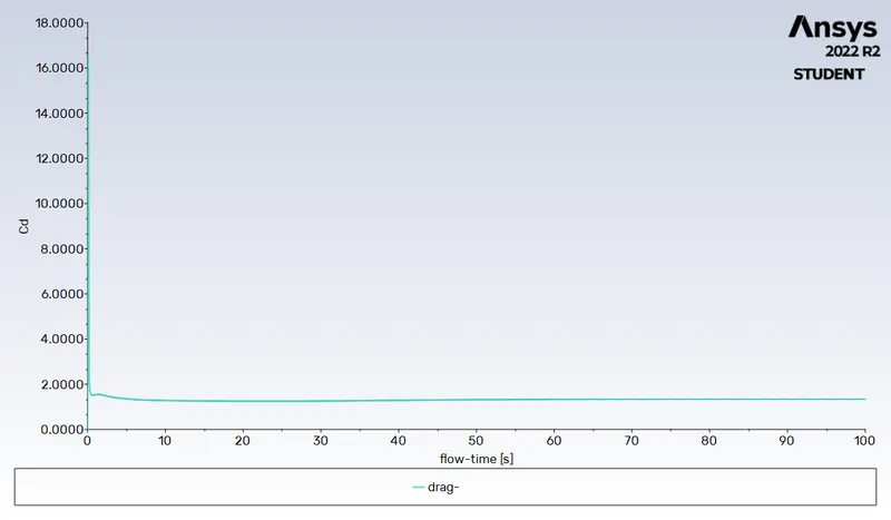
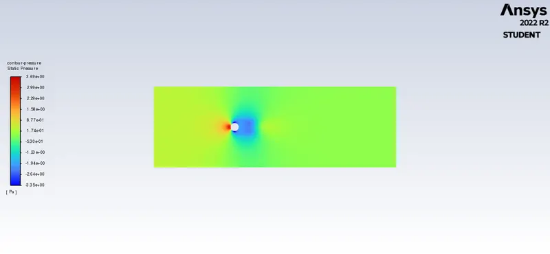
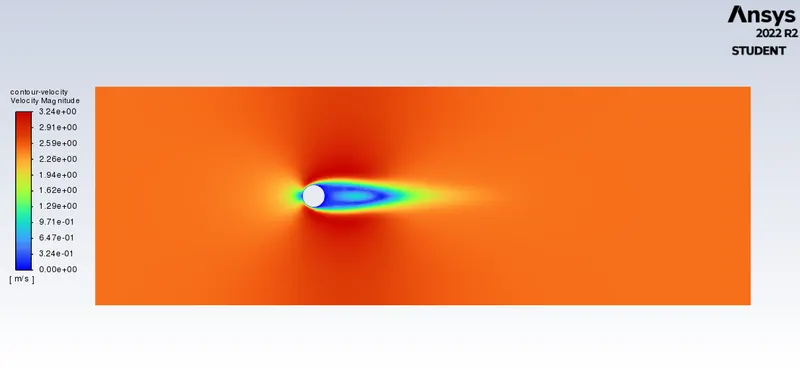
Steady state
Re =10
v=0.25
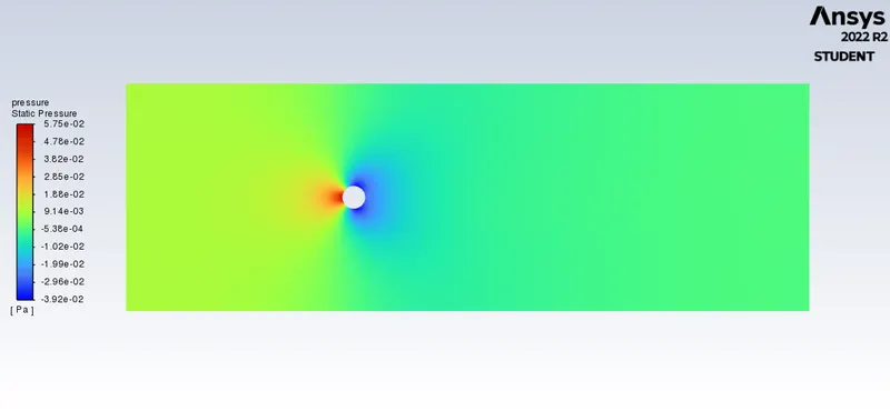
Steady state Re=1000
V=25m/s
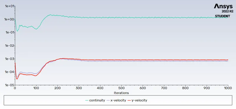
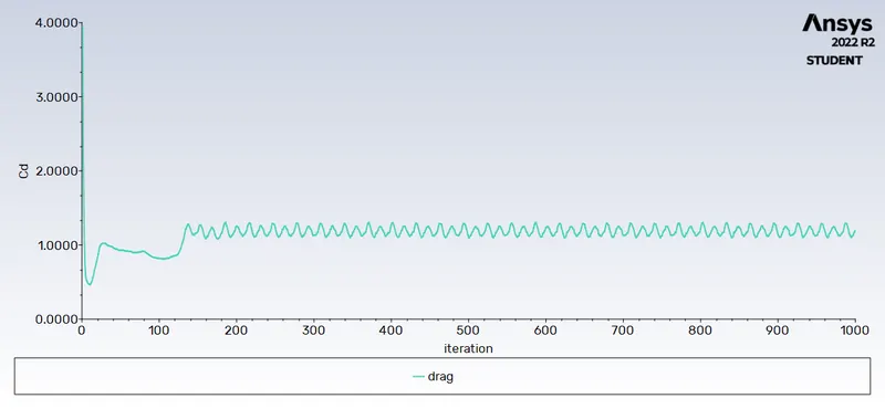
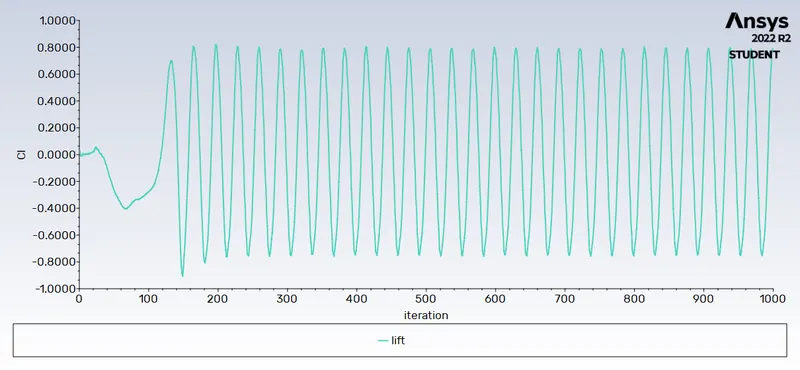
Re=10000
v=250m/s
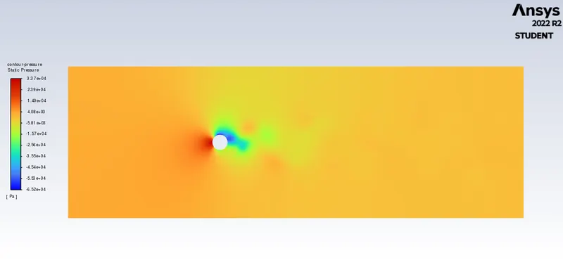
Re=100000
velocity=2500m/s
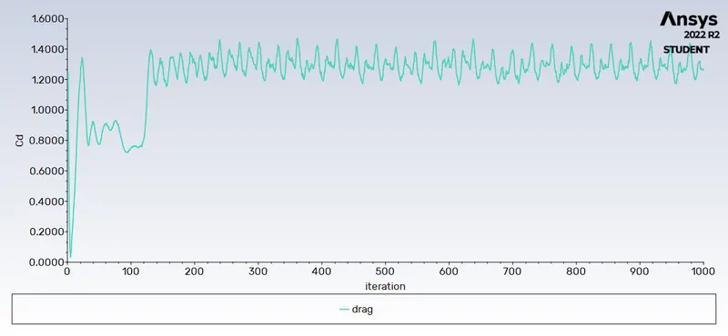
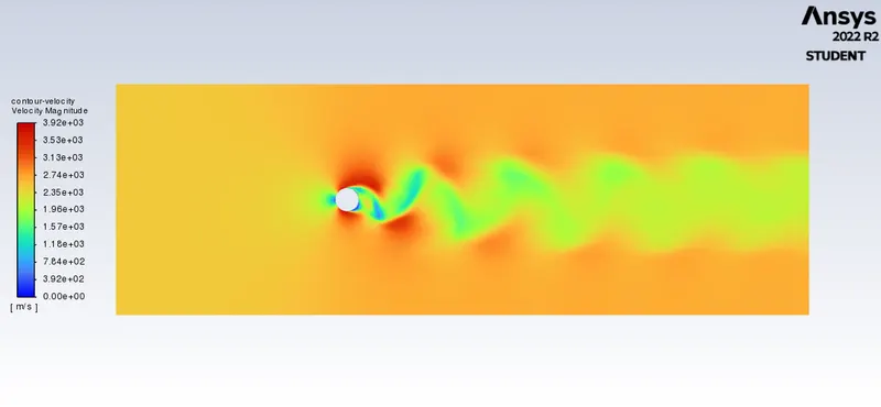
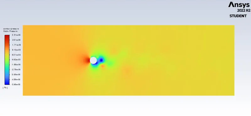
Validation
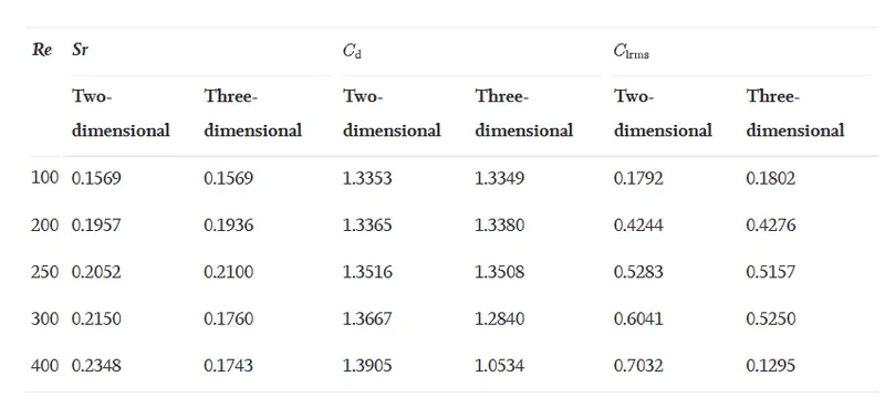
Results
| Re number | Velocity m/s | Viscocity | Drag cofficient | Lift cofficient | Vertex avarage veleocity m/s |
| 10 | 0.25 | 0.05 |
3.3305 |
-0.000366 |
0.1 |
| 100 | 2.5 | 0.05 |
1.3282 |
0.099 |
0.88 |
| 1000 | 25 | 0.05 |
1.041 |
-0.395 |
17.3 |
| 10000 | 250 | 0.05 |
1.12 |
-0.551 |
162 |
| 100000 | 2500 | 0.05 |
1.18 |
0.1288 |
1734 |
| usteady | 2.5 | 0.05 |
1.337 |
0.0544 |
1.51 |
Conclusion
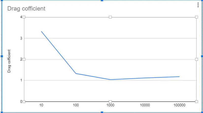
Drag cof vs Re
Looking at the above data We can come to conclusion That Drag cof is decresses as increse in the Ryenolds number
Refered matarial
https://www.sciencedirect.com/science/article/pii/S0307904X08000243