Week 2 - Flow over a Cylinder.

AIM: To Simulate the flow over a cylinder and explain the phenomenon of Karman vortex street.

OBJECTIVE:

• Performing 2D simulation.
• Modifying REYNOLDS NUMBER.
• Creating a customised fluid.
• Creating a run-time animations.
• Visualizing VORTEX SHEDDING.
• Adding monitor points.
• Creating animation files.
• Numerical diffusion.
• STEADY STATE VS TRANSIENT analysis.
• Post processing.

NEED TO PROVE:

PART-I

1. Simulate the flow with the steady and unsteady case and calculate the Strouhal Number for Re= 100.

PART-II

1. Calculate the coefficient of drag and lift over a cylinder by setting the Reynolds number to 10,100,1000,10000 & 100000. (Run with steady solver)
2. Discuss the effect of Reynolds number on the coefficient of drag. [ Results should be validated with any standard literature and error should be within 5 %]

STEPS TO SLOVE:

Open ansys >select fluid fluent.

GEOMETRY:

• Open geometry>file>space claim>options>units(meters)>ok.
• Select axis(Y)>select circle[dia=2M]>select rectangle[L=20M,B=60M].
• Select pull[surface created]>esc.
• Select option>delete circle>expand curves>select construction line>delete.

MESH:

Select mesh[right click]>select method>click automatic method>select geometry>apply>click method>select triangular>generate mesh>select sizing>select geometry>select type>number of divisions[36]>generate mesh>select infliation>geometry[face]>boundary[circle]>inflation option[first layer thickness,1st layer height[5e-003M]]>generate mesh>maximum layers[6]>update>gave names by select face and click N option[wall,inlet,outlet,symmetry boundary condition]>update.

SETUP:

• Double click on setup>double pression>parallel>4 processors>ok.
• Goto physics>select & keep steady,pressure based,absolute>goto viscous>laminar>select materials>fluent fluid materials[air],name as user-materials>density[[1kg/m3]>viscosity[0.05kg/m-s]>ok.
• cell zones>edit>select user-materials>ok.
• boundaries>inlet>edit>velocity[1m/s]>ok>outlet>edit>gaugepressure[0 pascal]>wall>edit>shear condition[no slip]>wall motion[stationary wall]>ok>symmetry>set as symmetry.
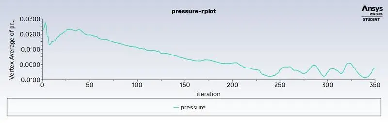
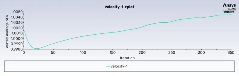
• Definations>surface report>vertex average>name as monitor point>post processingg>create>point>select point>create co-ordinates[x=8,y=0]>solving>definations>surface report>vertex average>field variable[velocity and velocity magnitude]>select monitor point>report file,report plot[create]>ok.
• Before initialization>select hybrid[method].
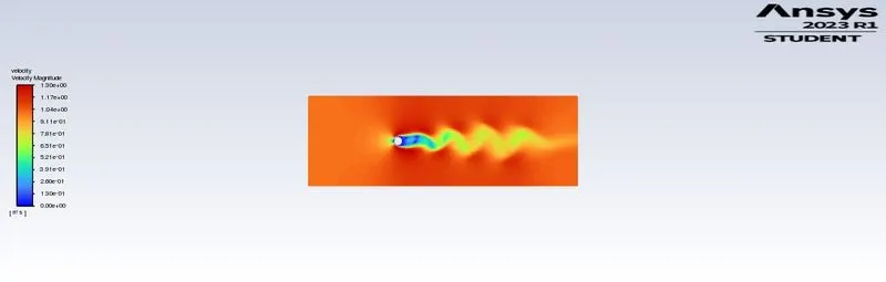
• post-processing>contours>new>contour name[velocity]>options[filled]>contours of[velocity],select all>save & display>compute>repeat for pressure.
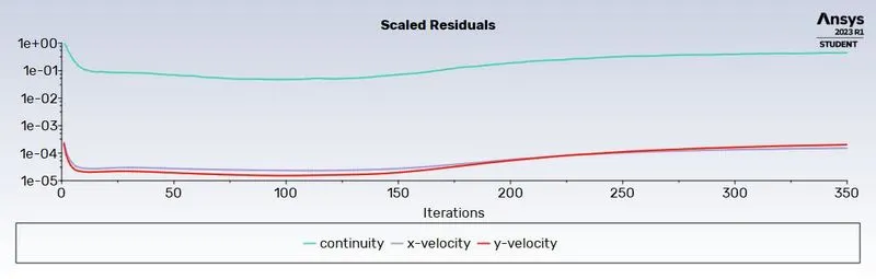
• solving>solution method>scheme[simple]>residuals>uncheck convergence>ok>iterations[350]>calculate.
• activites>createa>animations>name[velocity]>record after[10]>calculate.
• repeat the process for the unsteady by using re 100.

RESULTS:

STEADY STATE RE 10:

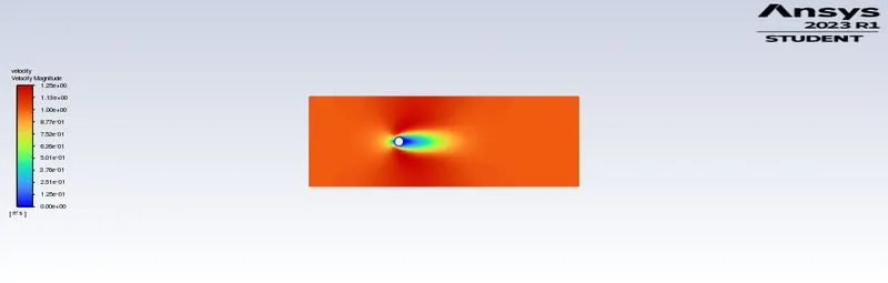
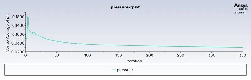
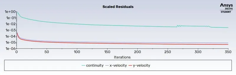
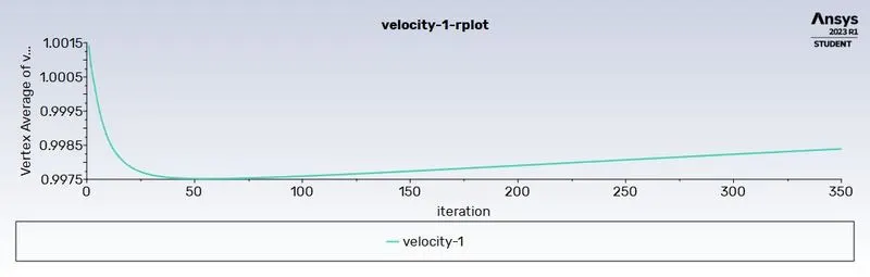
STEADY STATE RE 100:

STEADY STATE RE 1000:

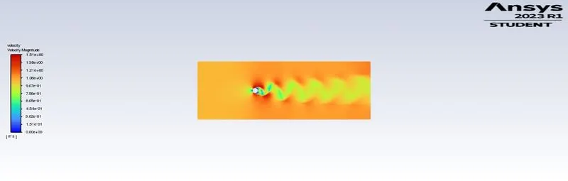
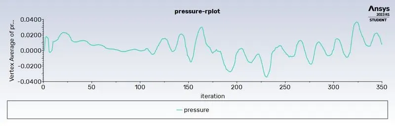
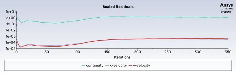
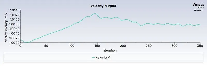
STEADY STATE RE 10000:

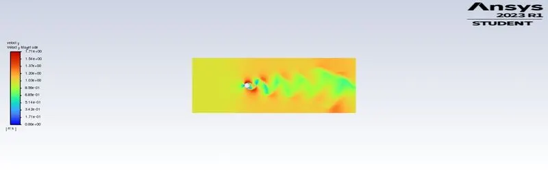
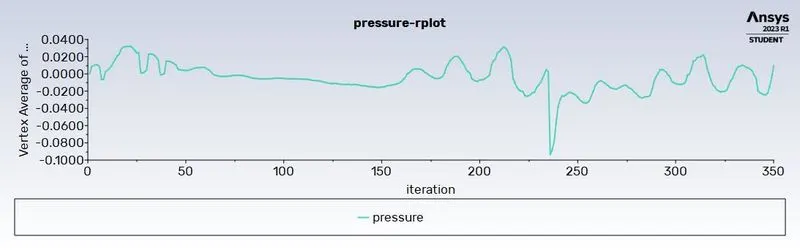
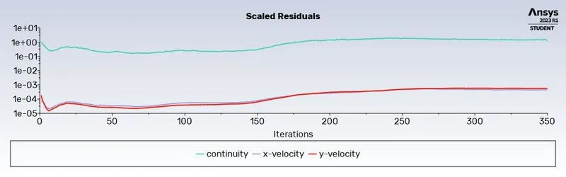
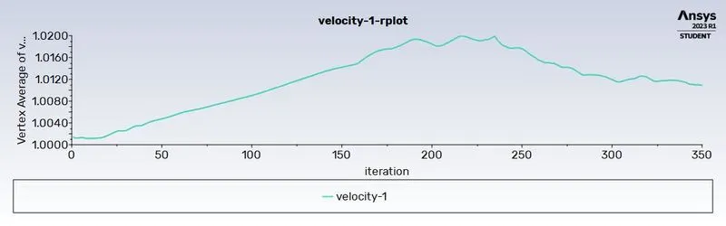
STEADY STATE RE 100000:

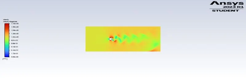
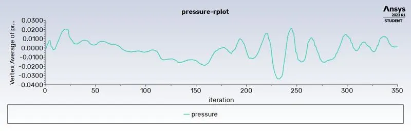
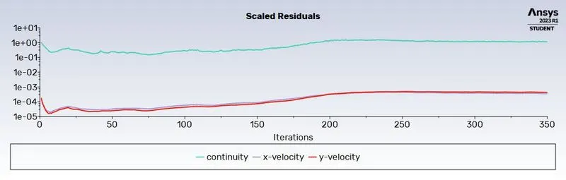
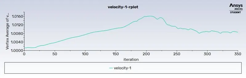
UNSTEADY STATE RE 100:

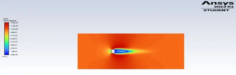
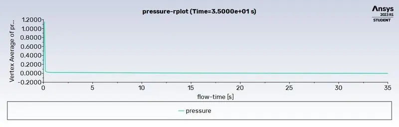
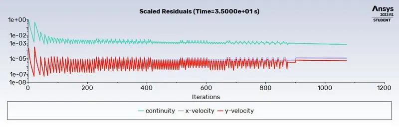
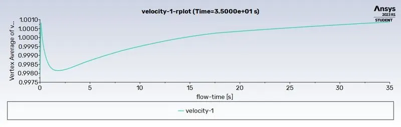
TABLE:

REYNOLDS NUMBER	MYU	VELOCITY	PRESSURE	STATE
10	0.2	0.99839239	0.39715385	STEADY
100	0.02	1.0044588	-0.0022005787	STEADY
1K	0.002	1.0076621	0.0075767738	STEADY
10K	0.0002	1.0109391	0.0093687209	STEADY
100K	0.00002	1.0085574	0.0013605803	STEADY
100	0.02	1.000867	-0.0016212292	UNSTEADY