Week 2 - Flow over a Cylinder.
FLOW OVER CYLINDER
AIM: Simulate the flow over a cylinder and explain the phenomenon of Karman vortex street.
PART-I:
Simulate the flow with the steady and unsteady case and calculate the Strouhal Number for Re = 100.
PART-II
- Calculate the coefficient of drag and lift over a cylinder by setting the Reynolds number to 10,100,1000,10000 & 100000 (using steady solver).
- Discuss the effect of Reynolds number on the coefficient of drag.
THEORY:
Vortex shedding:
- Vortex shedding is an oscillating flow that takes place when a fluid such as air or water flows past a body at certain velocities, depending on the size and shape of the body.
- During this, the vortices are created at the back of the body which detach periodically from either side of the body forming a Von Karman Street.
- Von Karman Street is a repeating pattern of swirling vortices, caused by a process known as vortex shedding, which is responsible for the unsteady separation of flow of a fluid around blunt bodies.
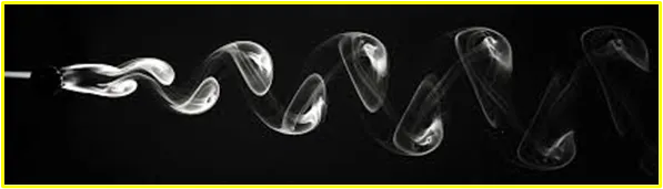
- A Von Karmen Street is formed only at a certain range of flow velocities, specified by a range of Reynolds Number (Re), typically above 40.
Strouhal Number:
It is a dimensionless number which describes the oscillating flow mechanisms. It is given by,
St = f L/u where,
f = frequency of vortex shedding
L = characteristic length (m)
u = flow velocity (m/s)
Y+:
Y+ is a dimensionless term which is used to determine if there is a need of wall function to be used in the simulation. Generally, a value of 10 or less is used if there is a viscous sub-layer and a value of 30-300 greater for turbulent region.
PART I: SIMULATION OF FLOW OVER CYLINDER USING STEADY AND UNSTEADY STATE AND CALCULATION OF STROUHAL NUMBER FOR Re = 100.
PROCEDURE:
GEOMETRY CREATION:
- Create a new project ‘Fluid flow (fluent)’ and double click to open Space Claim.
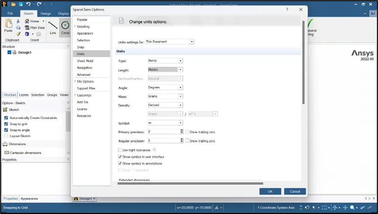
- Click on ‘file’ and select ‘space claim options.’ Click on ‘units’ and set it to ‘meters.’
-
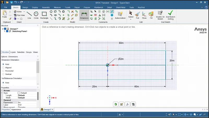
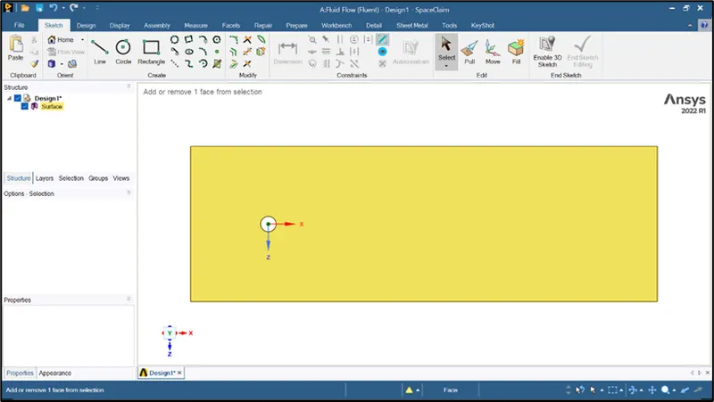
- Create a 2D geometry with a circle having 2 m diameter. Use construction lines to create a computational volume.
- Create ‘inlet’ at a distance ‘10D=20m’ from the centre of the cylinder and outlet at a distance ‘20D=40m. The ‘inlet’ and ‘outlet’ must be of dimension ‘10D’ separated by a distance of 60 m.
- After creation of geometry, click on ‘pull’ tool to convert it into a surface. Now click on ‘select’ tool and select and delete the circle.
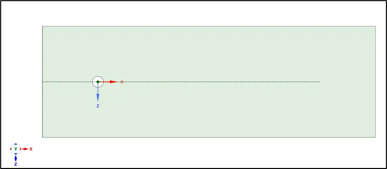
- Now select all the ‘construction lines’ in the ‘curves’ and delete them to complete the geometry.
MESH:
- Double click on ‘mesh’ to launch ‘Ansys Mesher.’
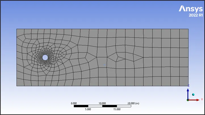
- The default mesh shows that the elements are quadrilateral in nature which is changed to triangular by inserting a method.
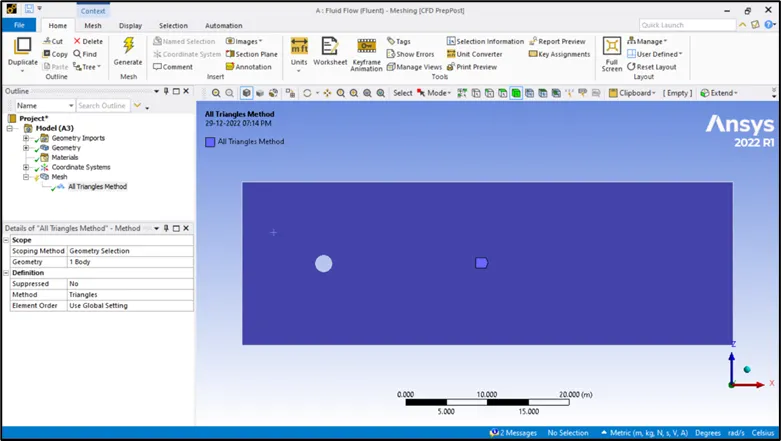
- Right click on ‘mesh’, click on insert and select ‘method.’
- Select the geometry and click on apply, and change the method to ‘triangles.’ Set the mesh element size to 25m and click on update mesh.
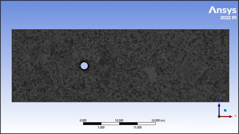
- As we zoom in to the surface of cylinder, it is observed that the geometry is not uniform which will affect the flow when simulated. This is resolved by using ‘sizing’ option under ‘mesh.’
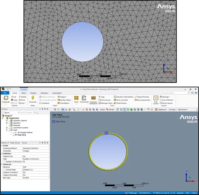
- Now update the mesh to obtain a smoother mesh around the cylinder surface.
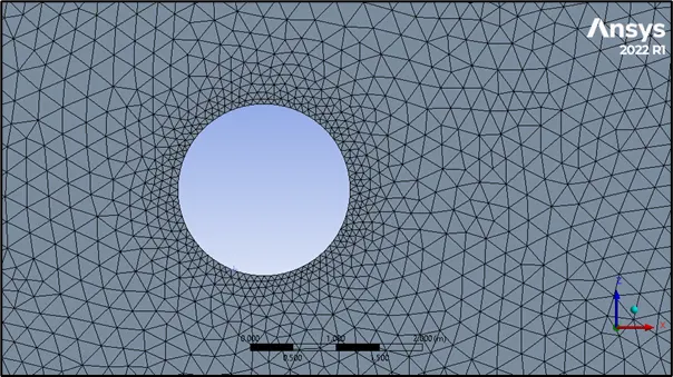
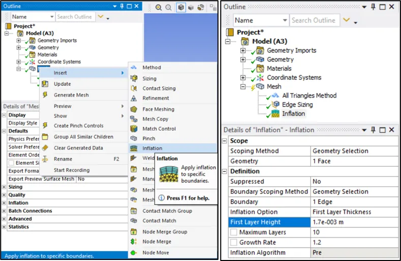
- Next step is to insert the inflation layers. The first layer thickness is decided based on the Y+ number, i.e., lesser than 10 for laminar flow (Re<2000) and 30 – 300 for turbulent flow (Re>2000).
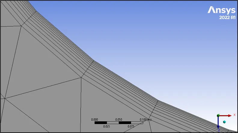
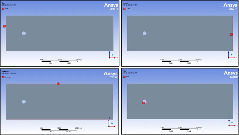
- Next step is to assign the named selection to the geometry.
SOLVER SETUP:
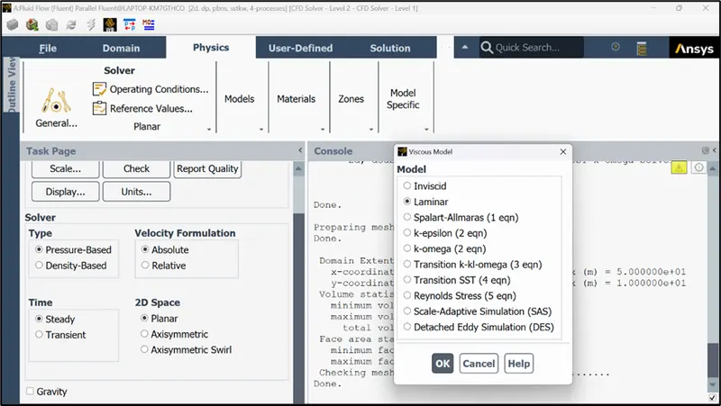
- Physics setup: - steady state, pressure-based solver and absolute velocity formulation.
- Viscous laminar flow model
MATERIAL CREATION:
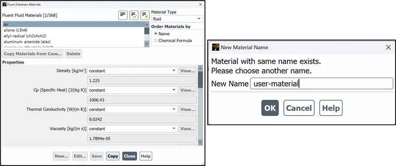
- Click on ‘fluent database’ and select ‘air’ and click on copy.
- Rename it as ‘user defined’ material and click OK.
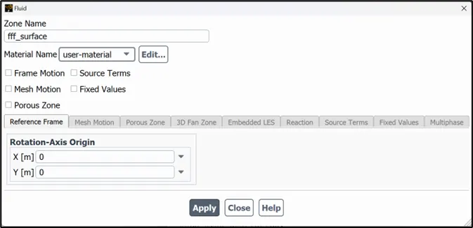
- The ‘air’ material will be auto assigned which is not required. To delete this first assign ‘user-material’ in cell zone volume (fff_surface) and click OK.
- Set the properties of the ‘user-material’ as ‘density = 1 Kg/m3’ and ‘viscosity = 0.02 Kg/m-s
- Now under ‘create/change material’ select ‘air’ and delete it.
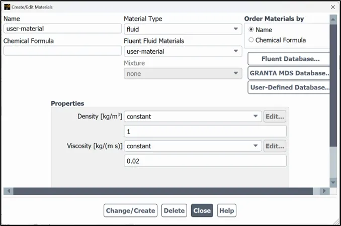
- Click on ‘change/create’ and close.
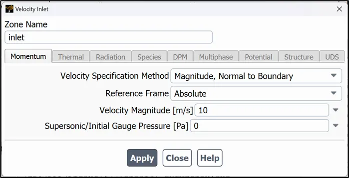
NOTE: THE BOUNDARY CONDITION (VELOCITY) IS THE ONLY VARIABLE THROUGH ALL DIFFERENT CASES WHICH ARE CALCULATED AND SHOWN FOR EACH CASE. THE OUTLET AND THE WALL HAS DEFAULT BOUNDARY CONDITIONS.
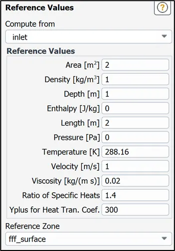
- Click on refence values and select compute from ‘inlet’ and reference zone ‘fff_surface.’
Creation of monitor point:
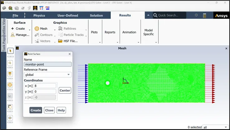
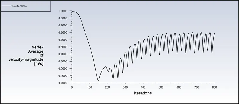
- Switch to post processing tab and create a point at a distance of ‘4D = 8m’ to right of cylinder to observe the variation of velocity.
SOLVING:
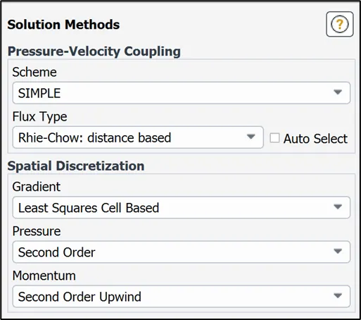
Solution method
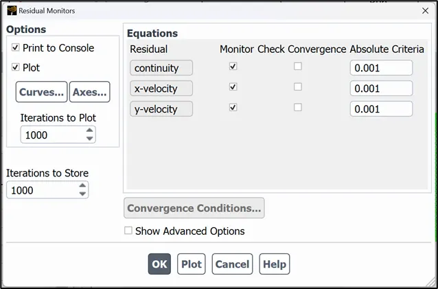
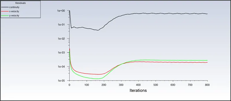
- Open ‘residual monitor’ and uncheck the convergence criteria of all the equation residuals.
REPORT DEFINITIONS:
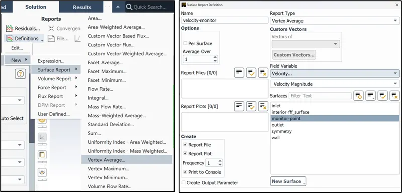
Surface report for velocity
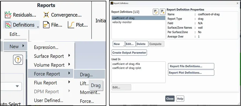
Report definition for coefficient of drag
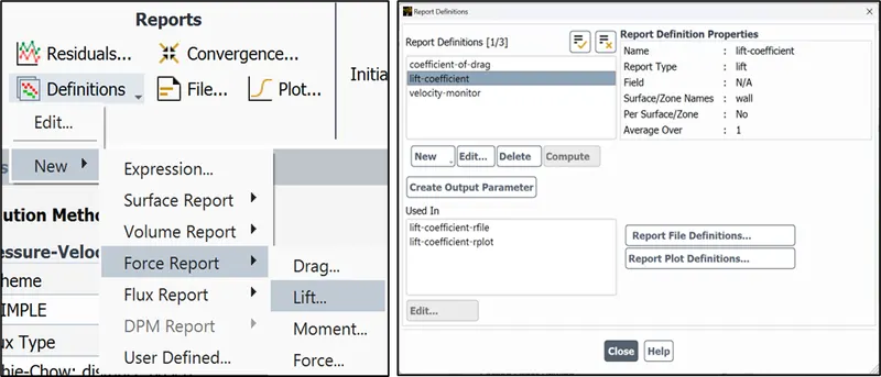
Report definition for lift
- Initialize the solution using ‘hybrid’ method.
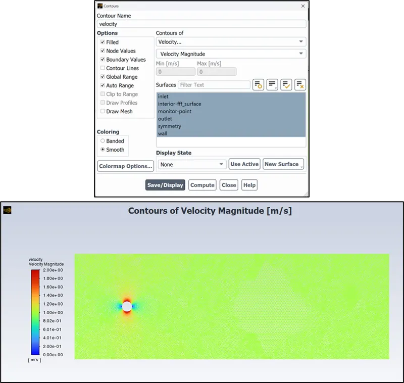
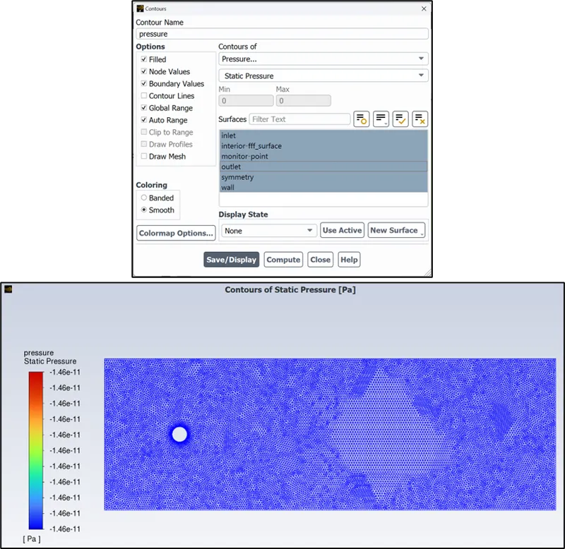
- In order to setup the contours, click on ‘results’, ‘contours’ under ‘graphics’ option.
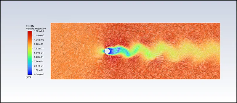
Velocity contour:
- This shows the value of velocity obtained due to hybrid initialization
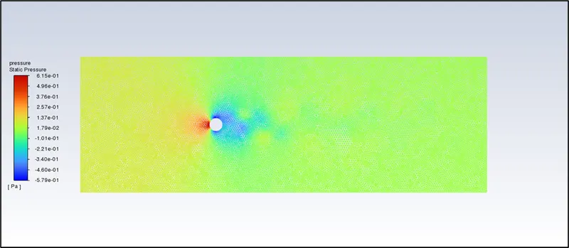
Pressure contour
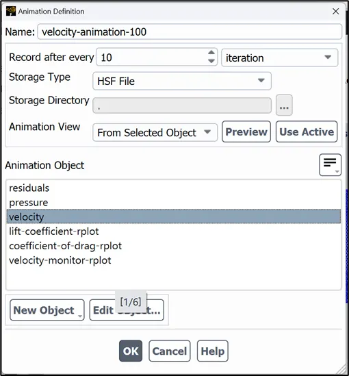
- To create an animation of the solution, click on create ‘solution animation’.
- Again, initialize the solution and run the simulation for 800 iterations.
PART 1: SIMULATE THE FLOW WITH THE STEADY AND UNSTEADY CASE AND CALCULATE THE STROUHAL NUMBER FOR RE = 100.
CASE 1: STEADY STATE SIMULATION

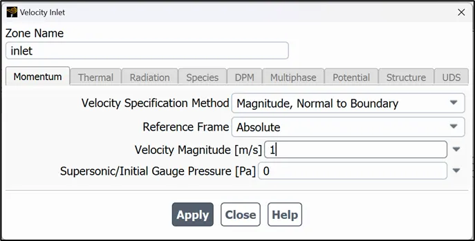
Inlet boundary condition:
Residual plot
Velocity monitor plot
Velocity animation
https://drive.google.com/file/d/1Zd3qC46T22b-982bkPSBUj289cm9idN3/view?usp=sharing
Velocity monitor plot
Velocity contour
Pressure contour
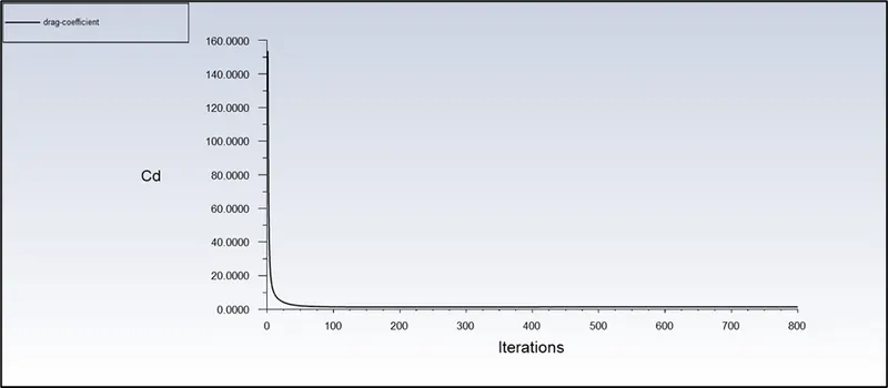
Drag coefficient = 1.3711
Lift coefficient plot
CASE 1: TRANSIENT STATE SIMULATION
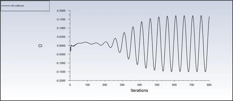
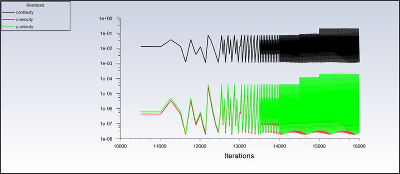
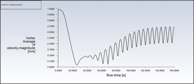
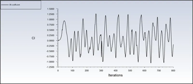
The simulation is run for 800 iterations with a time step of 0.2 with 20 iterations per time step.
Residual plot
Velocity monitor plot
Velocity contour
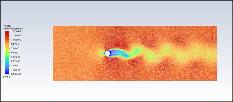
Velocity animation
https://drive.google.com/file/d/1XW2kV_6AjI1cVmohn231O9QRoQOlg8Nx/view?usp=sharing
Pressure contour
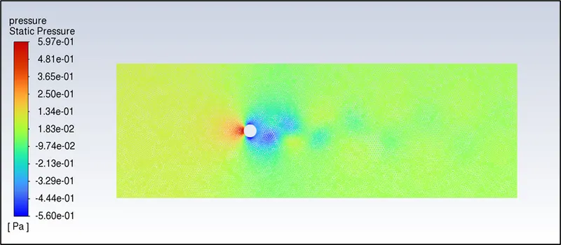
Drag coefficient = 1.3702
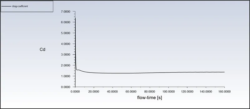
Lift coefficient
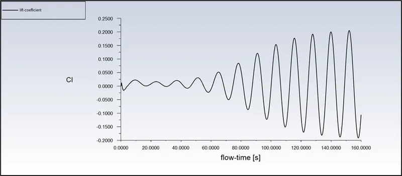
- The Strouhal number represents the frequency of Von Karman effect and can be calculated using the relation.

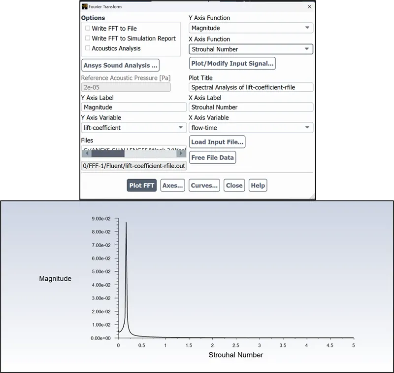
- Select ‘FFT’ plots and change the y axis function to ‘magnitude’ and x axis function to ‘Strouhal number’ and load the input file ‘lift-coefficient-rfile.out’ and click plot FFT.
- Enabling the ‘write FFT to file’ to obtain the data in ‘.txt or .xls’ format and the Strouhal number corresponding to the highest magnitude is the required value.
St = 0.162 (from the excel data)
Therefore,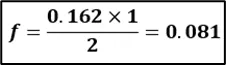
PART 2. SIMULATE THE FLOW WITH THE STEADY STATE FOR REYNOLDS NUMBER 10, 100, 1000, 10000 AND 100000 AND DISCUSS THE EFFECT OF REYNOLDS NUMBER ON COEFFICIENT OF DRAG
CASE 1. Re = 10

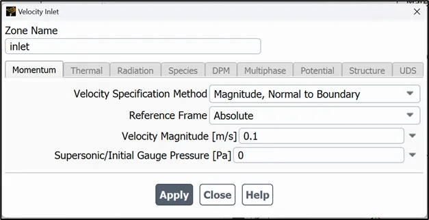
Inlet boundary condition
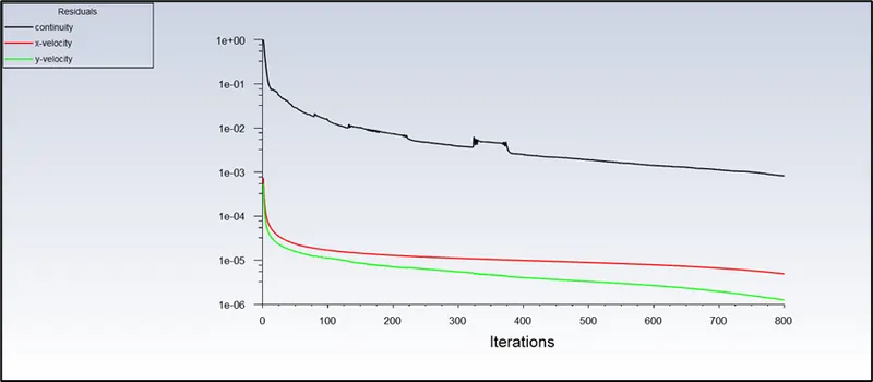
Residual plot
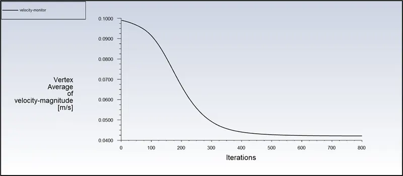
Velocity monitor plot
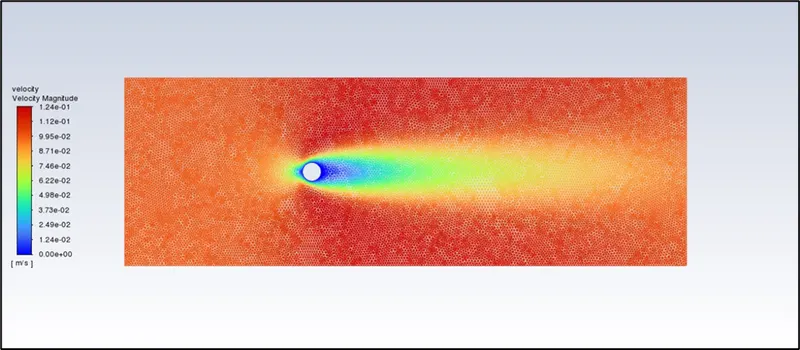
Velocity contour
Velocity animation
https://drive.google.com/file/d/1LE8cJBysrApu0YctvFsxfXXMm93Us-ZT/view?usp=sharing
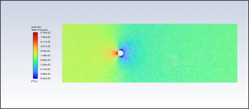
Pressure contour
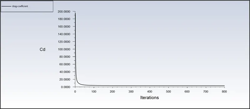
Drag coefficient = 3.3304
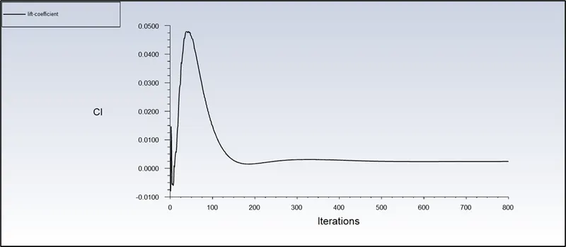
Lift coefficient
CASE 2. Re = 100
The results are similar and shown in part 1 steady state simulation.
CASE 3. Re = 1000

Inlet boundary condition
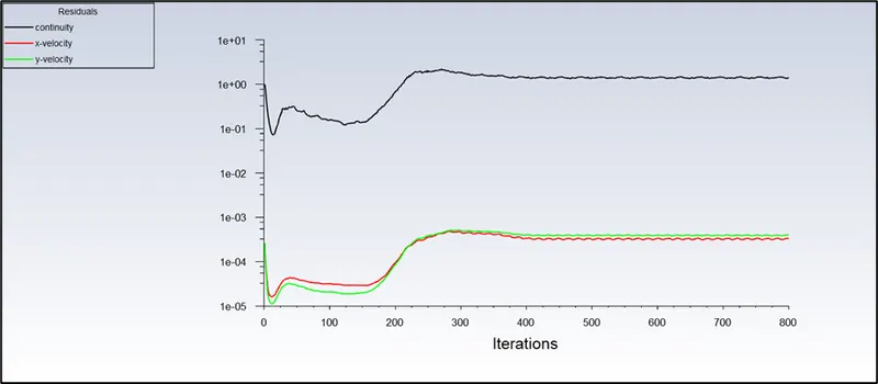
Residual plot
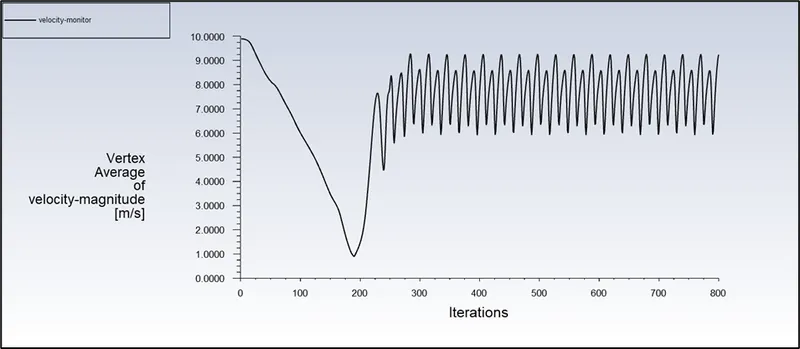
Velocity monitor plot
Velocity contour
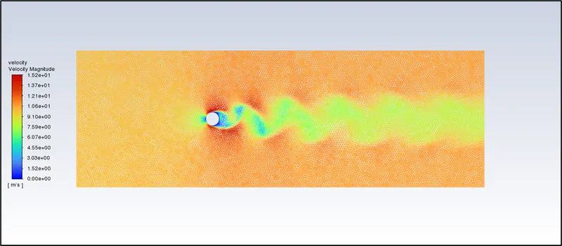
Velocity animation
https://drive.google.com/file/d/1cmriegFN4cy9RT-1nqH36BuwP3pLMBmV/view?usp=sharing
Pressure contour
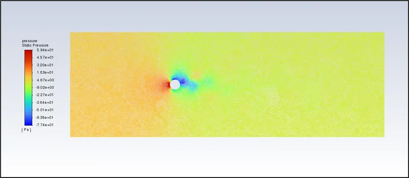
Drag coefficient = 1.2063
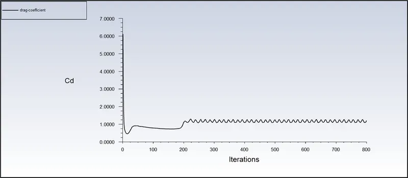
Lift coefficient
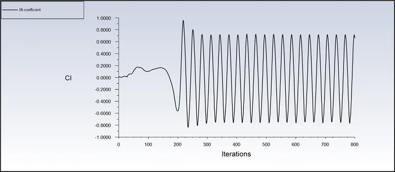
CASE 4. Re = 10000

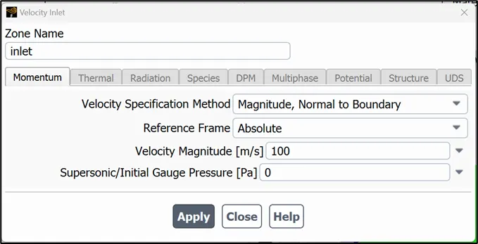
Inlet boundary condition
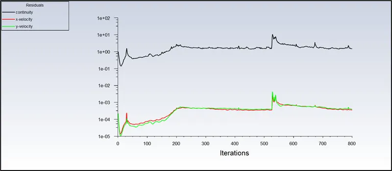
Residual plot
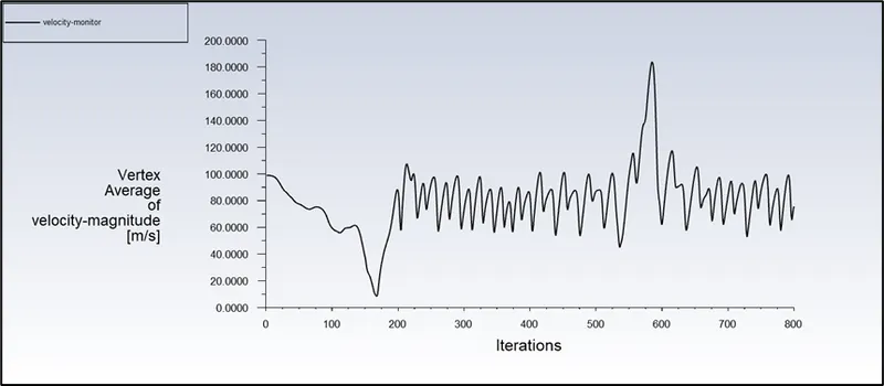
velocity monitor
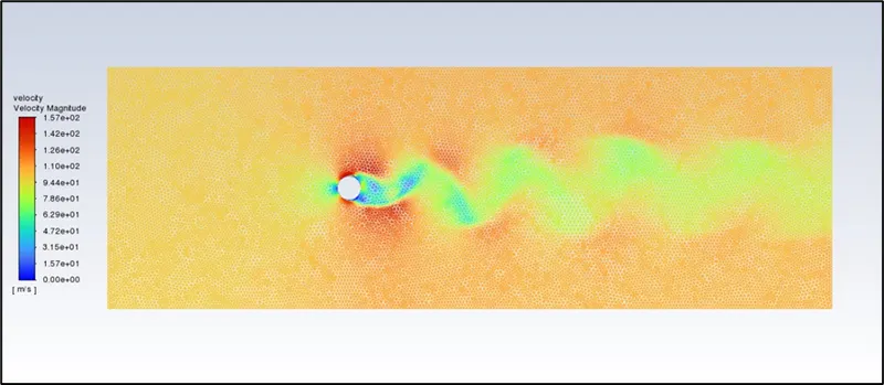
Velocity contour
velocity animation
https://drive.google.com/file/d/10puy-fLLPwe4rPNnz-pL1Ba-2eLXEjNJ/view?usp=sharing
pressure contour
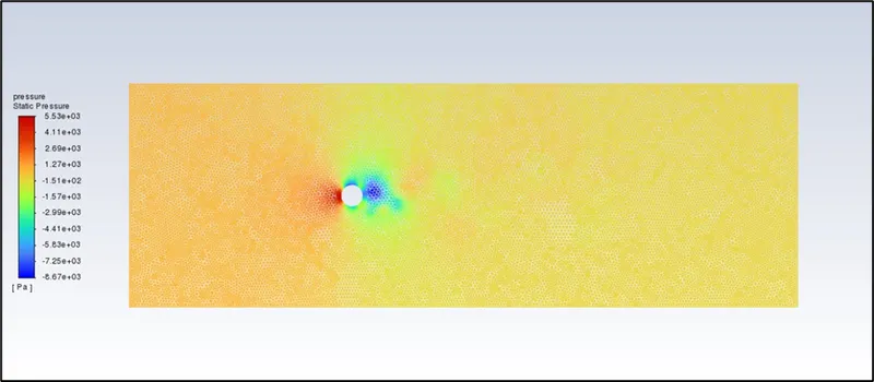
Drag coefficient = 1.003
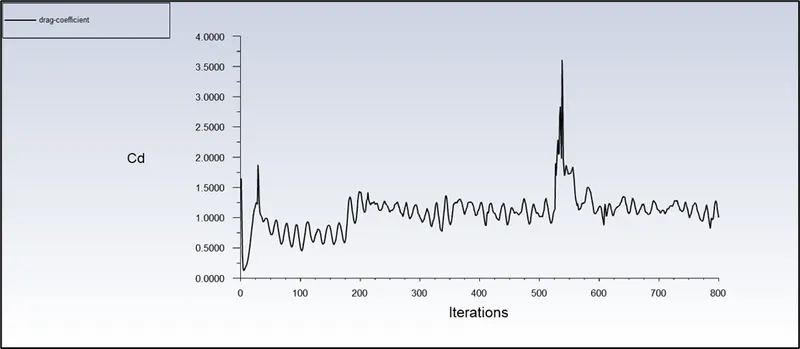
Lift coefficient
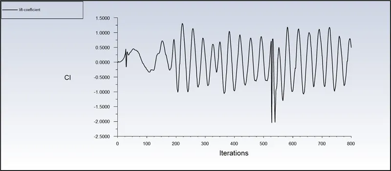
CASE 5. Re = 100000

Residual plot
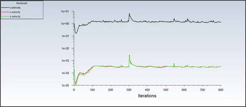
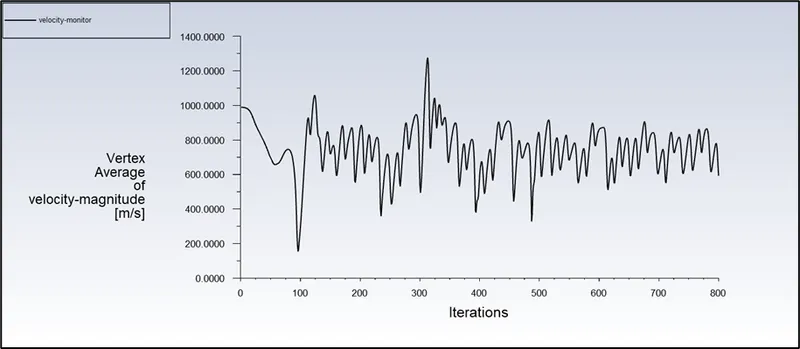
Velocity monitor
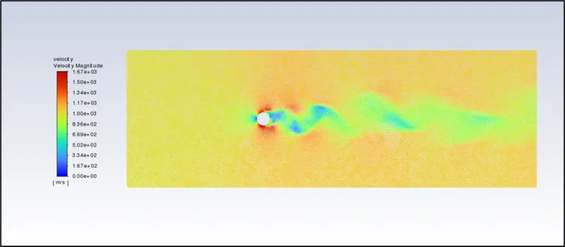
Velocity contour
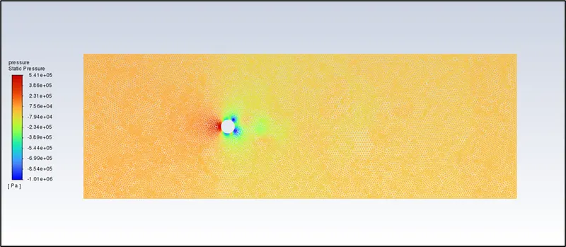
Pressure contour
Velocity animation
https://drive.google.com/file/d/1-ODboQCw7KFvip7TO8ivatz7ET4SGuLC/view?usp=sharing
Drag coefficient = 1.1806
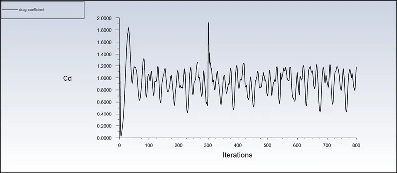
Lift coefficient
|
Reynolds number |
Velocity (m/s) |
Drag coefficient |
|
10 |
0.1 |
3.3304 |
|
100 (steady) |
1 |
1.3711 |
|
100 (transient) |
1 |
1.3702 |
|
1000 |
10 |
1.2063 |
|
10000 |
100 |
1.0030 |
|
100000 |
1000 |
1.1806 |
CONCLUSIONS:
- The drag coefficient decreases as the Reynolds number is increased.
- The Von Karman effect is not observed for Re = 10, because it is lesser than the critical Re for Von Karman effect to be observed.
- The Strouhal number obtained using transient study is 0.162.
- The drag coefficient at Re = 100 for steady and transient study are 1.3711 and 1.3702.
- Comparing transient results with a research study gives acceptable errors of 2.5% for drag coefficient and 3.1% for Strouhal number.
REFERENCES
https://www.sciencedirect.com/science/article/pii/S0307904X08000243