Simulation of a Flow over a Cylinder using ANSYS Fluent
Week 2 Report
- Aim: To perform a simulation for the flow over a cylinder for various cases and understand the process of Vortex Shedding.
- Theoretical Introduction:
In fluid dynamics, a Kármán vortex street (or a von Kármán vortex street) is a repeating pattern of swirling vortices, caused by a process known as vortex shedding, which is responsible for the unsteady separation of flow of a fluid around blunt bodies.
It is named after the engineer and fluid dynamicist Theodore von Kármán and is responsible for such phenomena as the "singing" of suspended telephone or power lines and the vibration of a car antenna at certain speeds.
A vortex street will form only at a certain range of flow velocities, specified by a range of Reynolds numbers (Re), typically above a limiting Re value of about 90. The (global) Reynolds number for a flow is a measure of the ratio of inertial to viscous forces in the flow of a fluid around a body or in a channel, and may be defined as a nondimensional parameter of the global speed of the whole fluid flow:

where:
 = the free stream flow speed (i.e. the flow speed far from the fluid boundaries like the body speed relative to the fluid at rest, or an inviscid flow speed, computed through the Bernoulli equation), which is the original global flow parameter, i.e. the target to be non-dimensionalised.
 = a characteristic length parameter of the body or channel
 = the free stream kinematic viscosity parameter of the fluid, which in turn is the ratio:

between:
 = the reference fluid density.
 = the free stream fluid dynamic viscosity
For common flows (the ones which can usually be considered as incompressible or isothermal), the kinematic viscosity is everywhere uniform over all the flow field and constant in time, so there is no choice on the viscosity parameter, which becomes naturally the kinematic viscosity of the fluid being considered at the temperature being considered. On the other hand, the reference length is always an arbitrary parameter, so particular attention should be put when comparing flows around different obstacles or in channels of different shapes: the global Reynolds numbers should be referred to the same reference length. This is actually the reason for which the most precise sources for airfoil and channel flow data specify the reference length at the Reynolds number. The reference length can vary depending on the analysis to be performed: for a body with circle sections such as circular cylinders or spheres, one usually chooses the diameter; for an airfoil, a generic non-circular cylinder or a bluff body or a revolution body like a fuselage or a submarine, it is usually the profile chord or the profile thickness, or some other given widths that are in fact stable design inputs; for flow channels usually, the hydraulic diameter about which the fluid is flowing.
For an aerodynamic profile, the reference length depends on the analysis. In fact, the profile chord is usually chosen as the reference length also for the aerodynamic coefficient for wing sections and thin profiles in which the primary target is to maximize the lift coefficient or the lift/drag ratio (i.e. as usual in thin airfoil theory, one would employ the chord, Reynolds, as the flow speed parameter for comparing different profiles). On the other hand, for fairings and struts the given parameter is usually the dimension of internal structure to be streamlined (let us think for simplicity it is a beam with a circular section), and the main target is to minimize the drag coefficient or the drag/lift ratio. The main design parameter which becomes naturally also a reference length is therefore the profile thickness (the profile dimension or area perpendicular to the flow direction), rather than the profile chord.
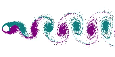
Karman vortex street Phenomena
Strouhal Number:In dimensional analysis, the Strouhal number (St, or sometimes Sr to avoid the conflict with the Stanton number) is a dimensionless number describing oscillating flow mechanisms. The parameter is named after Vincent Strouhal, a Czech physicist who experimented in 1878 with wires experiencing vortex shedding and singing in the wind. The Strouhal number is an integral part of the fundamentals of fluid mechanics.
The Strouhal number is often given as
where f is the frequency of vortex shedding, L is the characteristic length (for example, hydraulic diameter or the airfoil thickness) and U is the flow velocity. In certain cases, like heaving (plunging) flight, this characteristic length is the amplitude of oscillation. This selection of characteristic length can be used to present a distinction between Strouhal number and reduced frequency:
where k is the reduced frequency, and A is the amplitude of the heaving oscillation.
- Procedure:
1. The very first step is to create the Cross-section of the cylinder. To do this, we must use the Space claim that we have on the ANSYS workbench. Here, we draw the circle and then draw the inlet and Outlet of the domain. The Inlet is at a distance of 10D measured from the centre of the circle. The Outlet is at a distance of 20D from the centre of the circle. The diameter of the circle is 2m.
2. We then have to delete all the construction lines and use the pull command to convert the sketch to a surface. We just have to pull the sketch and convert it to a surface for our use.
3. After this is done, then next we need to input a mesh on the surface of the geometry that we have created. To insert the mesh, we need to use the module of Mesh in the Workbench. Here we add a few parameters so that we can control the mesh even better and get much more accurate results.
The parameters are, a.Sizing: using this parameter, we can better capture the circle by creating a certain number of divisions along the circumference of the circle. If we do not use these divisions, the circle will be captured more in the shape of a pentagon or a hexagon. So by creating the divisions, we are creating more nodes at the circumference and hence making the geometry much more circular.
b.Inflation layer: This parameter helps us create a body-fitted mesh and helps us control the mesh in a certain region.
c.Method: Here, we can control the Element size and the type of mesh that we deploy. In our case, the mesh type that we use is a triangular mesh with an average element length equal to 0.5m
4. Next we must name the edges for applying the Boundary condition. The edges can be named Inlet, Outlet and Symmetry. According to the names that we give, the solver then sets the Boundary condition for those particular sides.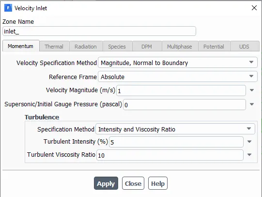
Inlet Boundary Condition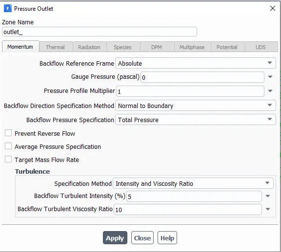
Outlet Boundary Condition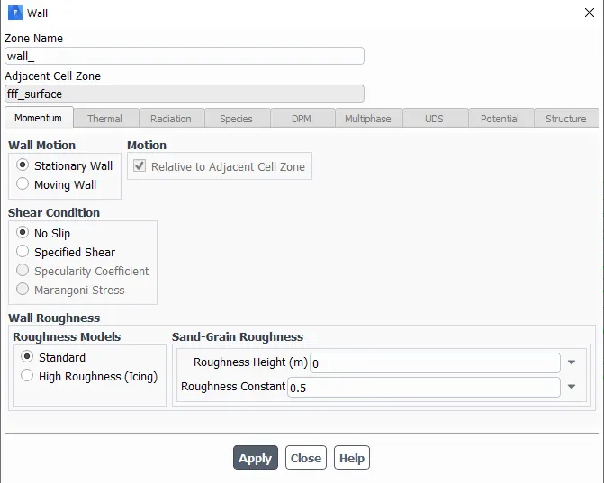
Cylinder Wall Boundary Condition
These are the Boundary conditions that we have given for the different types of Boundaries that we have created in the model.
5. The next step is to change the material property according to our need so that we can change the Reynolds number by varying the velocity of the flow of air over the cylinder. The reference values that we have used are as follows: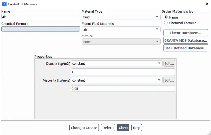
Material Property change
We have used the density of the material, in our case, it is air, as 1 kg/m3 and the viscosity as 0.05 kg/m-s. We know that
Reynolds Number = `(rho * u * L )/ (mu)`
So, if we vary the inlet air velocity, we will be varying the Reynolds number of the flow.
6.We also need to create the Coefficient of drag and the Coefficient of Lift plots from the simulations that we will be doing. We also need to find the velocity at a particular point at a particular distance away from the circle towards the outlet of the domain.
The coordinates of this point are (8,0) in the x-y axis.
To create these plots, we need to use the "definitions" tool and then create these plots and a report for these quantities as well. We then need to study these plots and draw conclusions from them.
7. We have various cases that we study under this assignment where we vary the Reynolds number by varying the Inlet Velocity. We vary the Reynolds Number from Re= 10,100,1000,10000,100000 by varying the type of solver and the Inlet Velocity according to the Reynolds number for which we are performing the simulation.
- Results:
a. Reynolds Number = 10
Simulation is done using the Steady state solver and keeping the Inlet velocity as the following:
Reynolds Number = `(rho * u * L )/ (mu)`
10 = (1) (u) (2) / (0.05)
here, we get u = 0.25 m/s
The plots are as following: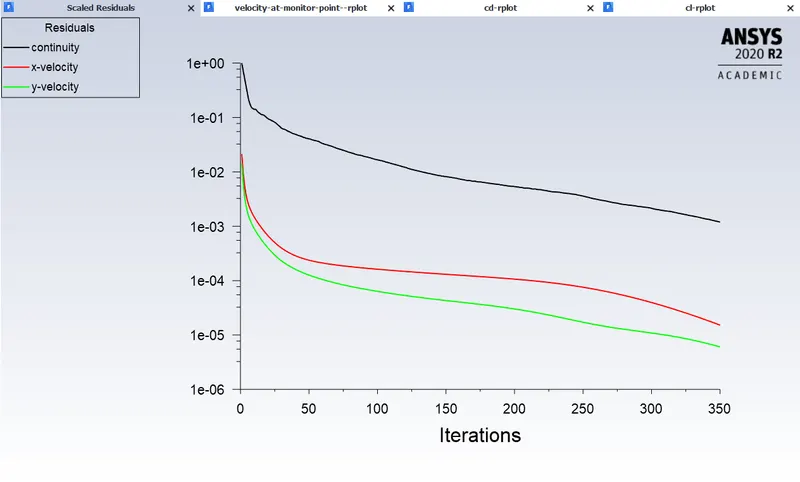
Scaled Residuals


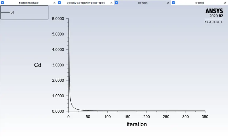
Coefficient of Drag Plot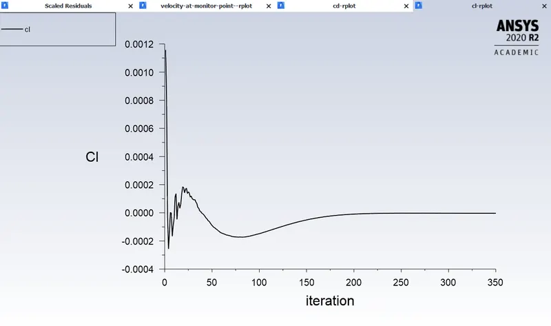
Coefficient of Lift Plot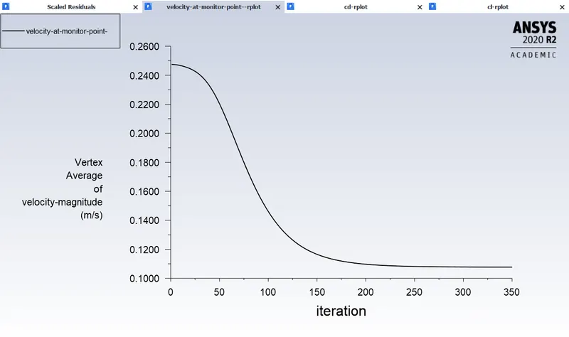
Velocity at the point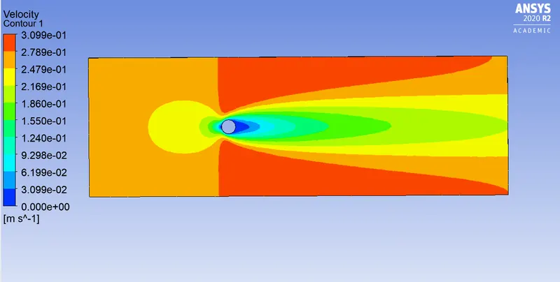
Velocity contour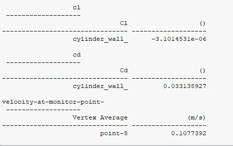
Cd, Cl and Velocity values
From the photo above, we can see that the value of `C_d` = -3.101e-6 , `C_l` = 0.03313, Velocity = 0.107 m/s
b. Reynolds Number = 100
b.1) Steady Solver
The simulation is done in the Steady Solver where we use the Reynolds Number formula to calculate the Inlet Velocity of the airflow.
Reynolds Number = `(rho * u * L )/ (mu)`
100 = (1) (u) (2) / (0.05)
u = 2.5 m/s
The plots are as follows: 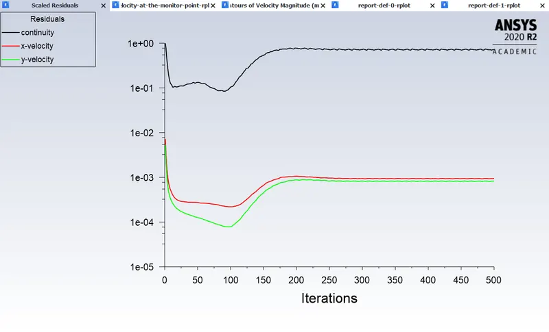
Scaled Residuals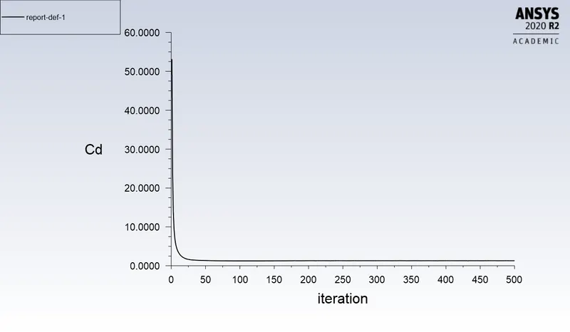
Coefficient of Drag Plot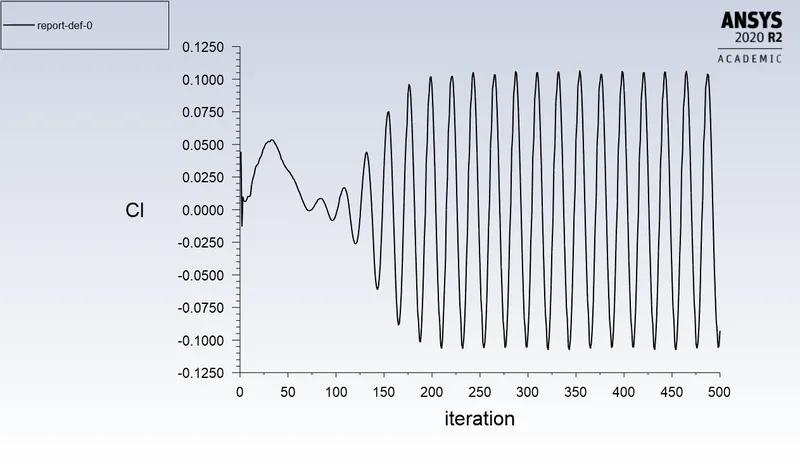
Coefficient of Lift Plot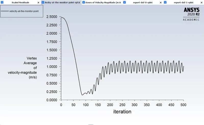
Velocity at the point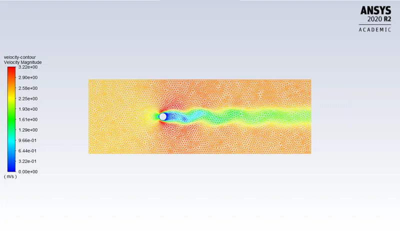
Velocity Contour
Here from the contour, we can see Vortex Shedding occurring in the domain. Vortex shedding can be confirmed from the Coefficient of Lift plot as well. In the Coefficient of Lift plot, we can see the oscillations in the values of it. These Osciallations confirm the occurrence of vortex shedding occurring in the domain. So, we can conclude that for Reynolds number there is an occurrence of Vortex Shedding for the given Geometry.
b.2) Re =100 with Transient Solver
In this case, we simply change the solver from Steady to Transient and give the time-step size and the number of Time-steps as well.
We get the following plots: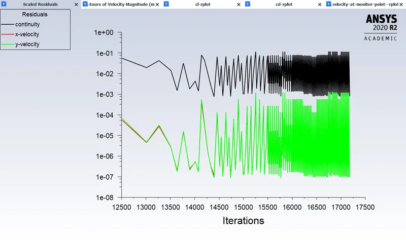
Scaled Residuals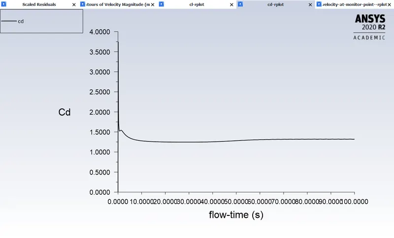
Coefficient of Drag Plot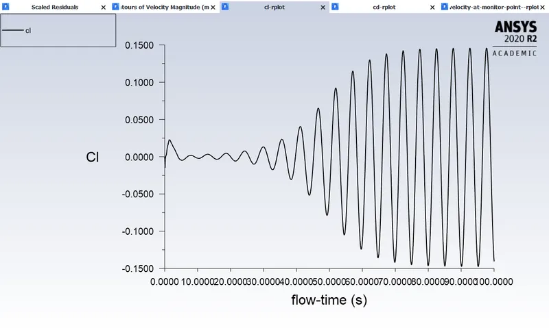
Coefficient of Lift plot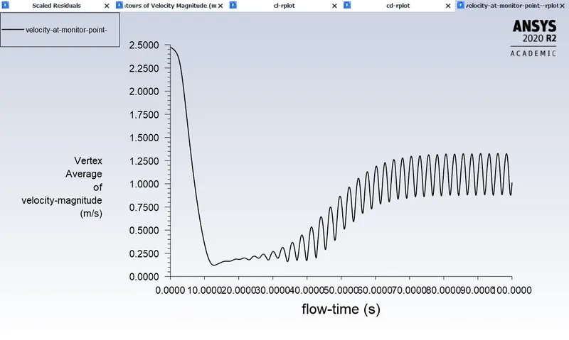
Velocity at the point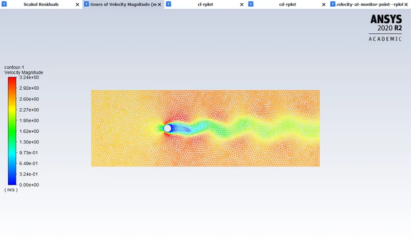
Velocity Contour
The Vortex shedding can be again seen in this case as well as it should. Because by simply changing the Solver type, the Physics of the problem should not change which can be seen in the plots of the two cases above. 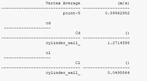
Values of Cd, Cl and velocity
Below is the video file for the flow over a cylinder.
c. Re = 1000
We again have to calculate the Inlet velocity, which will be:
Reynolds Number = `(rho * u * L )/ (mu)`
1000 = (1) (u) (2) / (0.05)
u = 25 m/s
The plots are as follows: 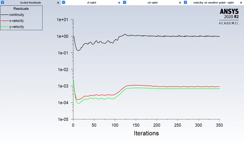
Scaled Residuals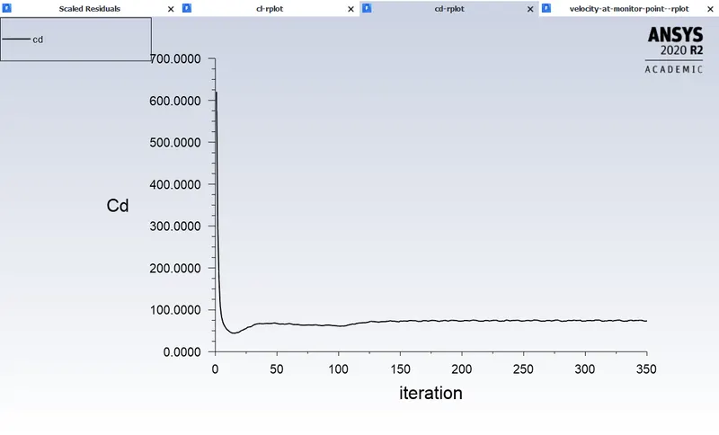
Coefficient of Drag plot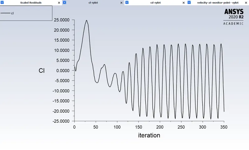
Coefficient of Lift plot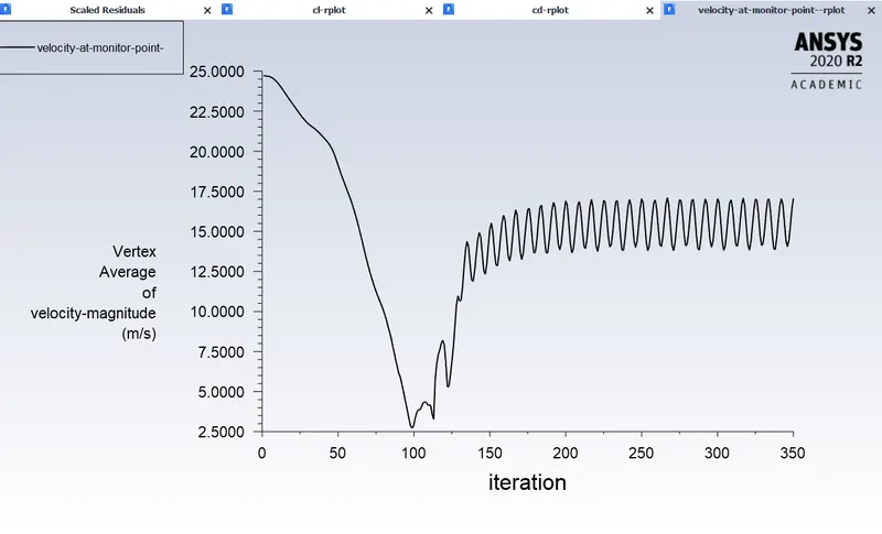
Velocity at the point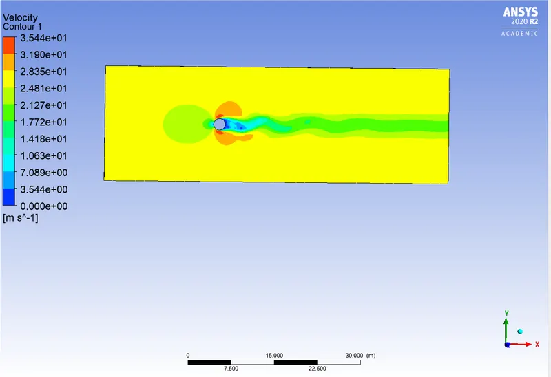
Velocity Contour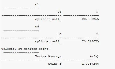
Values of Cd, Cl and Velocity
d. Re = 10000
Reynolds Number = `(rho * u * L )/ (mu)`
10000 = = (1) (u) (2) / (0.05)
u = 250 m/s
The plots are as follows: 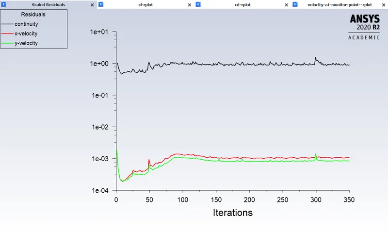
Scaled Residuals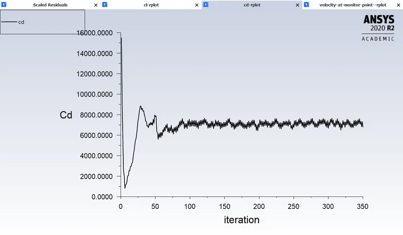
Coefficient of Drag plot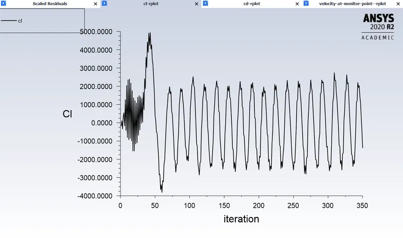
Coefficient of Lift plot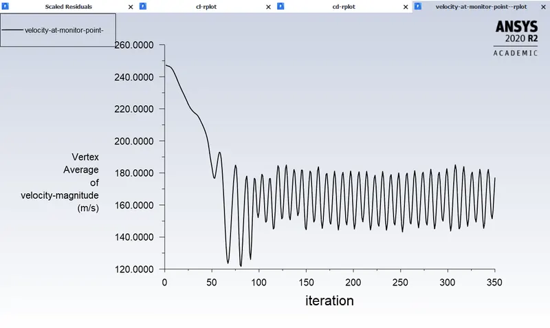
Velocity at the point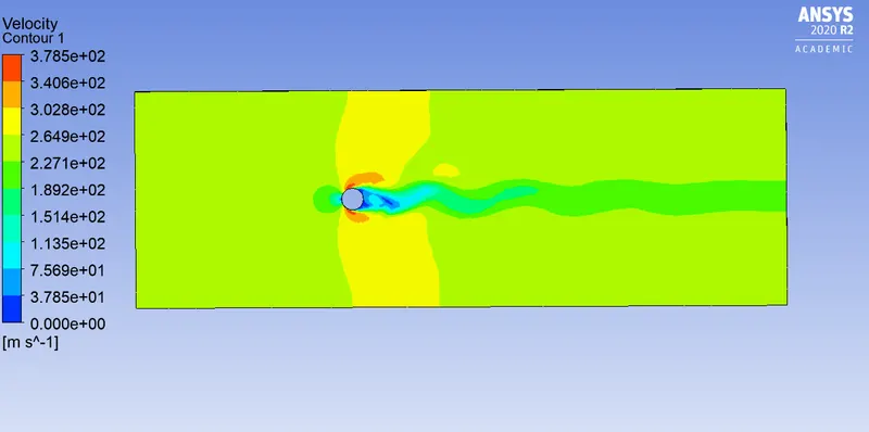
Velocity Contour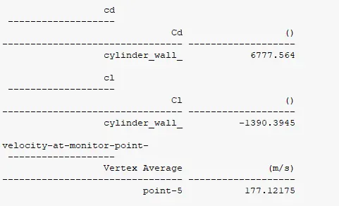
Values of Cd, Cl and velocity
d. Re = 100000
Reynolds Number = `(rho * u * L )/ (mu)`
100000 = = (1) (u) (2) / (0.05)
u = 2500 m/s
The plots are as follows: 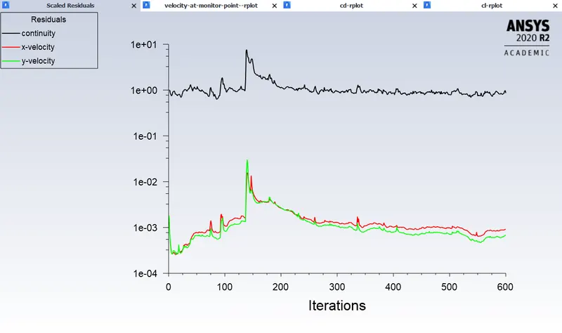
Scaled Residuals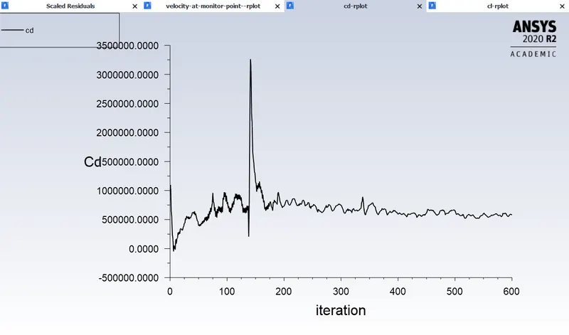
Coefficient of Drag plot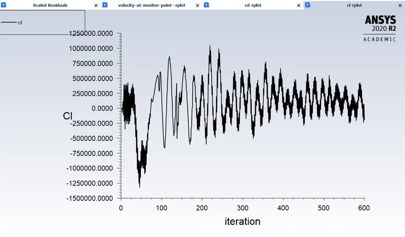
Coefficient of Lift Plot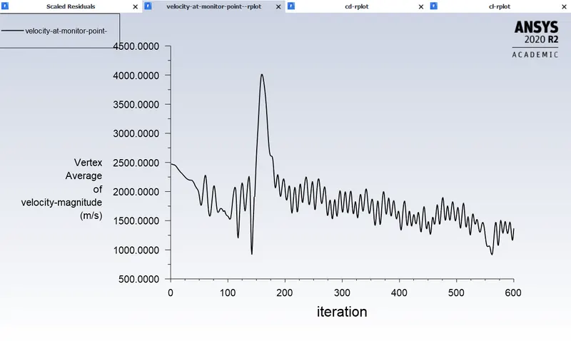
Velocity at the point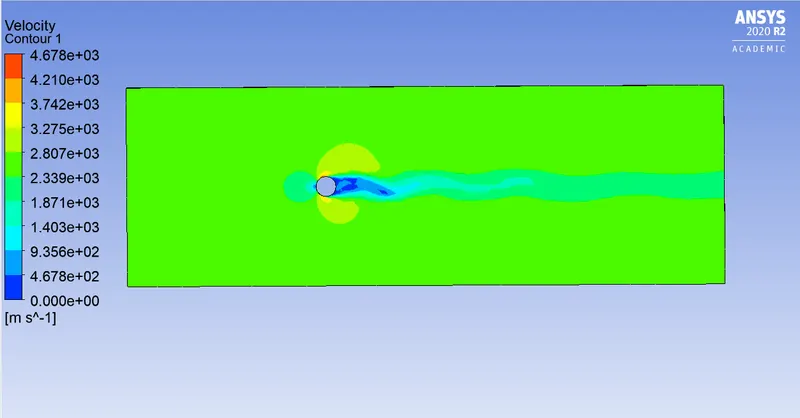
Velocity Contour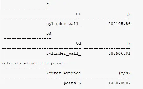
Values of Cd, Cl and Velocity
- Validation:
Reference Research Paper:- https://www.sciencedirect.com/science/article/pii/S0307904X08000243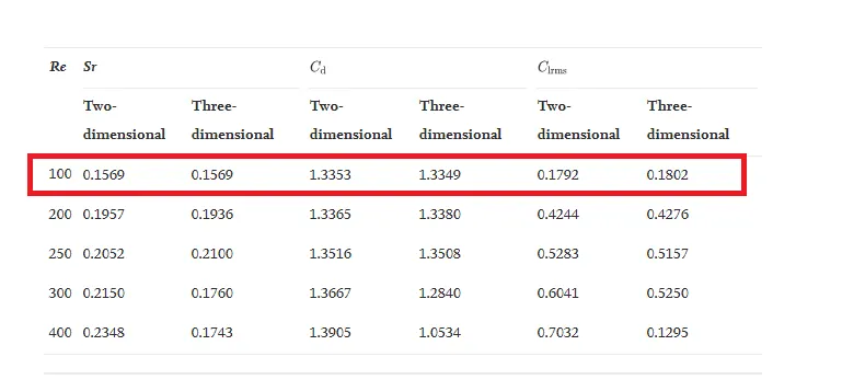
The Coefficient of Drag value that we get is 1.27 and the reference values are 1.3349.
Error = (1.3353-1.27) / (1.3353) = 0.0486 = 4.86% , which is below the limit
The value of the Strouhal Number that we get is 0.147 and whereas in the paper, the value that the author gets is 0.1569.
Error = (0.1569 - 0.147) / (0.1569) = 0.063 = 6.3% , which is again below the limit.
- Conclusions:
In conclusion, I would like to state that this challenge helped me gain a much better understanding of how to set up different cases in ANSYS Fluent and also helped me understand the different factors on which vortex shedding and turbulence occurs. We can see that in both the cases, i.e the steady-state simulation and the Transient state simulation have converged after having a look at the Scaled Residuals plot and the plot for the Coefficient of Lift. The Scaled Residuals have become stable after a certain number of iterations and the Coefficient of Lift plot is oscillating as expected. Hence we can conclude that the simulation has converged. We get the Vortex Shedding phenomena occurring after the Reynolds number goes above 47, in our case, which is 100,1000,10000,100000. All the Vortex Shedding can be confirmed in the Coefficient of lift plots for the simulation.