Week 2 - Flow over a Cylinder.
REPORT ON FLOW OVER A CYLINDER
AIM
To Simulate the flow over a cylinder and explain the phenomenon of Karman vortex street. Also,
PART-I
- Simulate the flow with the steady and unsteady case and calculate the Strouhal Number for Re= 100.
PART-II
- Calculate the coefficient of drag and lift over a cylinder by setting the Reynolds number to 10,100,1000,10000 & 100000. (Run with steady solver)
- Discuss the effect of Reynolds number on the coefficient of drag.
- Results should be validated with any standard literature and error should be within 5 %
THEORY
Kármán vortex street
In fluid dynamics, a Kármán vortex street (or a von Kármán vortex street) is a repeating pattern of swirling vortices, caused by a process known as vortex shedding, which is responsible for the unsteady seperation of flow of a fluid around blunt bodies. A vortex street will form only at a certain range of flow velocities, specified by a range of Reynold's Number (Re), typically above a limiting Re value of about 90. The Reynold's Number is calculated using the equation `Re = (rho*v*d)/nu`. For the wake of a circular cylinder, for which the reference length is conventionally the diameter d of the circular cylinder, the lower limit of this range is Re ≈ 47
where rho = density, v =velocity, d = diameter of the pipe and nu = dynamic viscosity of the fluid Reynold's Number states whether a flow is laminar or turbulent
When a single vortex is shed, an asymmetrical flow pattern forms around the body and changes the pressure distribution. This means that the alternate shedding of vortices can create periodic lateral (sideways) forces on the body in question, causing it to vibrate.
Strouchal Number
Strouhal number is a dimensionless number describing oscillating flow mechanisms.
The Strouhal number is often given as
`St = (fD)/(U')`
Where,
f= frequency of vortex shedding
D= characteristic diameter of the cylinder
U'= fluid flow velocity
Co-efficient of drag:
In fluid dynamics, the drag coefficient `(C_d)` is a dimensionless quantity that is used to quantify the drag or resistance of an object in a fluid environment, such as air or water. It is used in the drag equation in which a lower drag coefficient indicates the object will have a less aerodynamic or hydrodynamic drag. The drag coefficient is always associated with a particular surface area.
The drag coefficient of any object comprises the effects of the two basic contributors to fluid dynamic drag: skin friction and form drag. The drag coefficient of a lifting airfoil or hydrofoil also includes the effects of lift-induced drag. The drag coefficient of a complete structure such as an aircraft also includes the effects of interference drag.
The drag coefficient `(C_d)` is defined as`C_d = (2F_D)/(rhou^2A)`
Co-efficient of Lift
The lift coefficient `(C_L)` is a dimensionless coefficient that relates the lift generated by a lifting body to the fluid density around the body, the fluid velocity, and an associated reference area
`C_L = L/(qS) = (2L)/(rhou^2S ), where q = 1/2rhou^2`
L is the lift force,
S is the relevant surface area and
q is the fluid dynamic pressure, in turn, linked to the fluid density, and to the flow speed.
PROCEDURE
The first step is we open Ansys Fluent and create geometry which is shown below
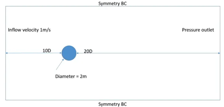
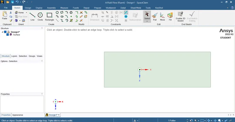
We create a 2D image of the geometry using the sketch tool as per the given geometric values.
Next step is to generate the mesh for that we open the meshing tool and we create the mesh which is in the shape of triangles using the insert method tool
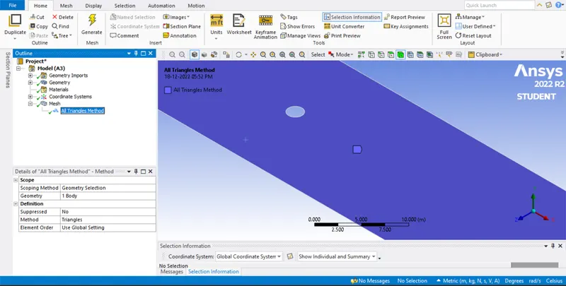
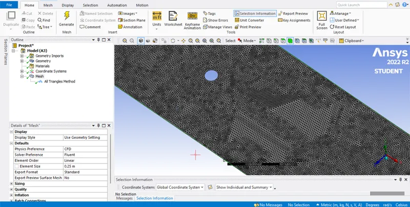
Then we need to reduce the corners of the circle that is being created to avoid inaccuracy using sizing tool
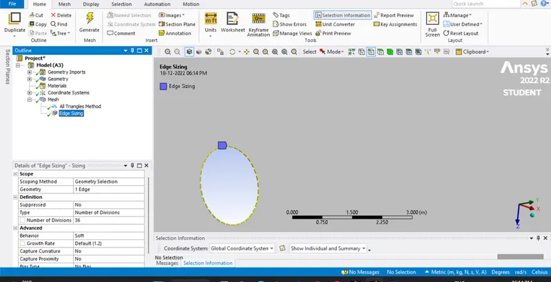
Now let us create the inflation layers because we also need the flow around the cylinder.
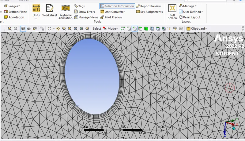
Now we set up the boundaries and solve it using the steady state condition at first and then unsteady state condition
For steady state condition we use the pressure based solver and calculate under steady state condition and with absolute velocity formulation.
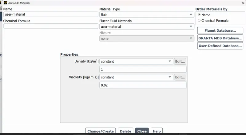
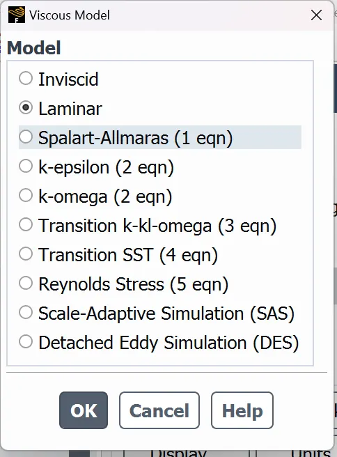
We use viscous model as Laminar because the flow is laminar. We also change the fluid name from air to user-material and then we give the initial density and viscosity values
Now let us create a Monitor point which is a point that is created at a few distance from the center of the ircle so that we ae able to view the change in the velocity.
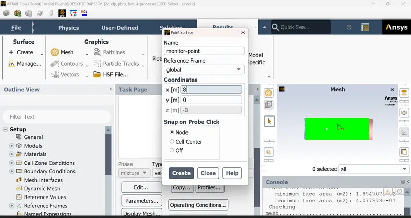
Then we create the vertex average plot of velocity for the monitor point and name it as monitor-point-velocity. The monitor point is created to check the velocity change. The point is created at a distance
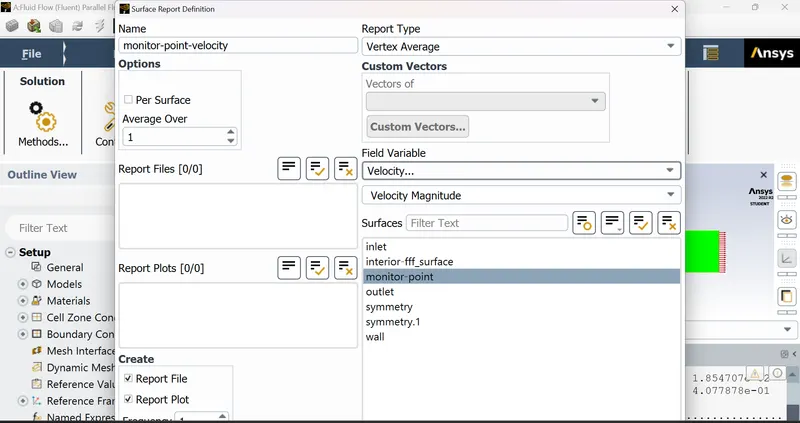
Then we find the vertex average at the monitor point and then we create the velocity and pressure contour plots.
For that first we initialize the set of equations and then set up the plots using the contour tool in results
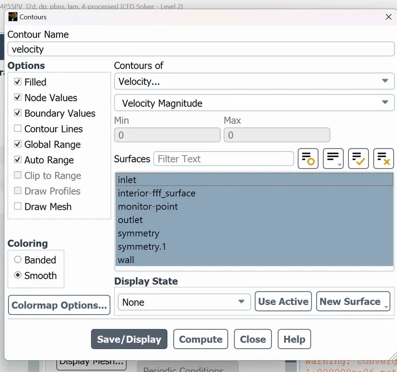
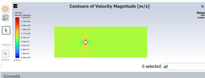
Similarly we create pressure contour which appears as shown below
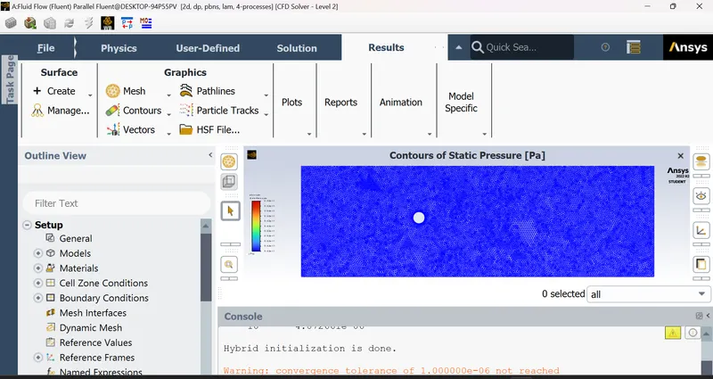
Then we switch back in solution and we use SIMPLE solution method and then we create the animation for velocity at the monitor point
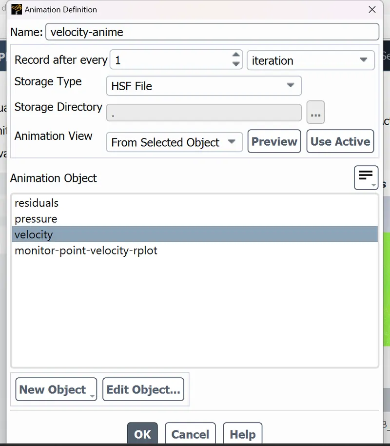
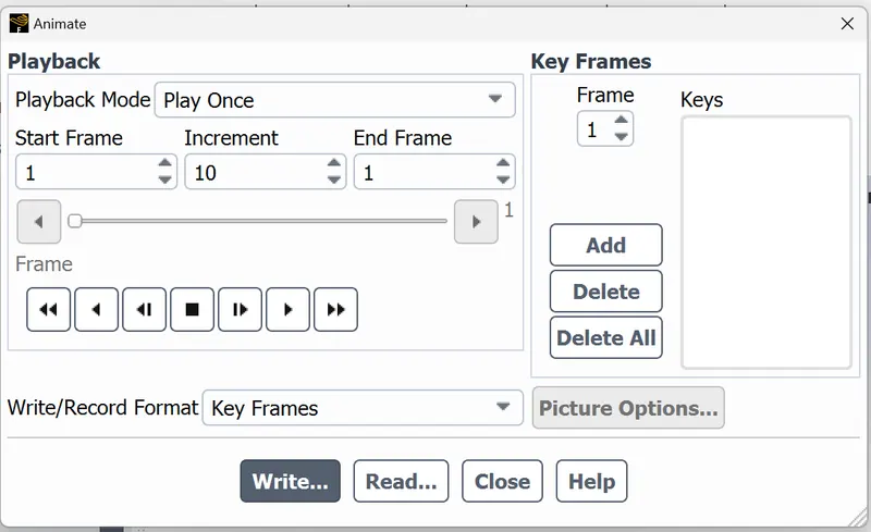
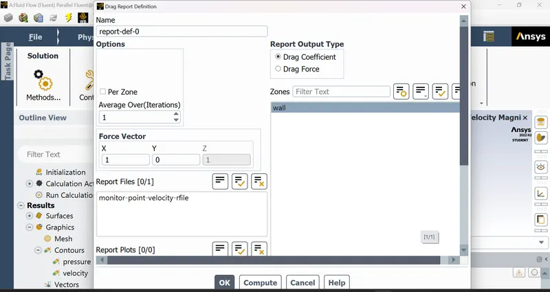
We are also asked to find the drag and lift cofficient. We generate the plot for drag and lift using the definition and creating the plot inside it
RESULTS
PART 1
Under Steady state Condition at Re = 100, Viscosity = 0.02 kg/m sec, velocity = 1 m/s, Diameter = 2 Number of iterations = 500 iterations
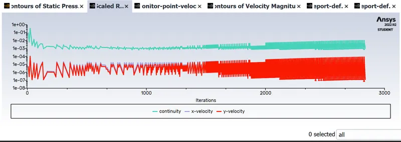
Residuals
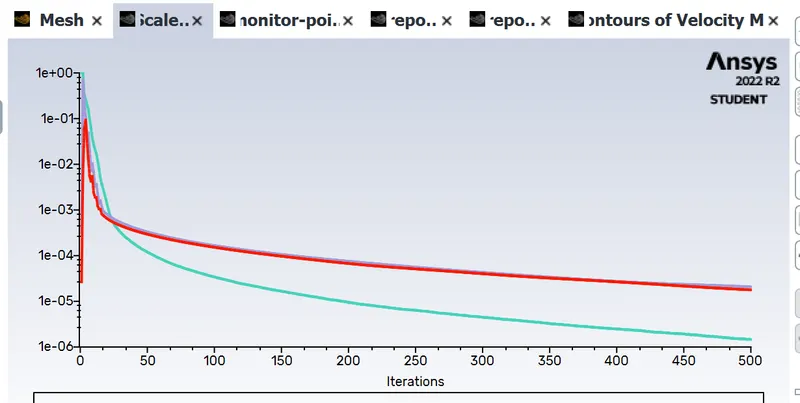
This plot helps in monitoring the change in each and every convergence criterion for every time step and plots those values for every iteration or time step. This plot helps to know when convergence is achieved.
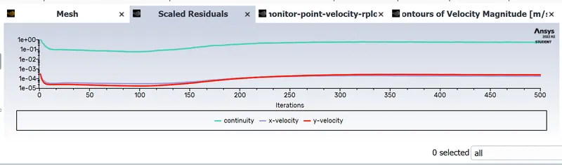
From the above plot, we can see that the solution has reached a steady state even before 500 iterations.
MONITOR POINT VELOCITY:
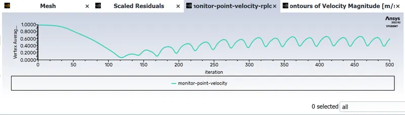
The average velocity is approximately 0.6 m/s
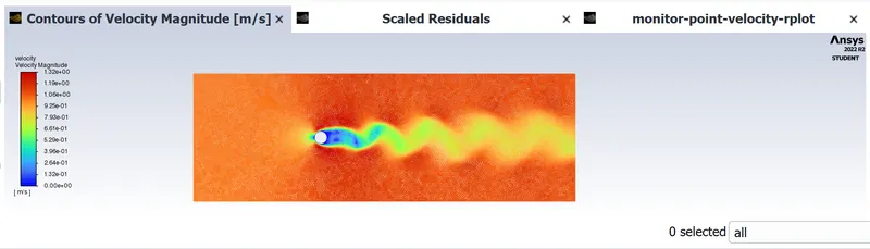
Velocity Contour
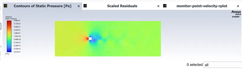
Pressure Contour
Coefficient Drag
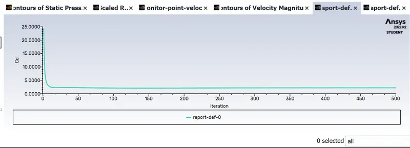
Coefficient of drag = 1.5105
Coefficient of Lift
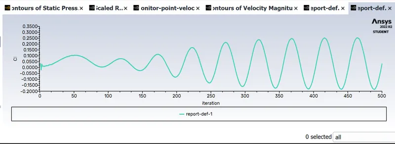
Coefficient of Lift = 0.2613
STROHAUL NUMBER:
The strohaul number cannot be calculated for the steady state as we don't calculate the flow with respect to time.
Under Transient state Condition
at Re = 100, Viscosity = 0.02 kg/m sec, velocity = 1 m/s, Diameter = 2 Number of time steps = 500
Residuals
MONITOR POINT VELOCITY:
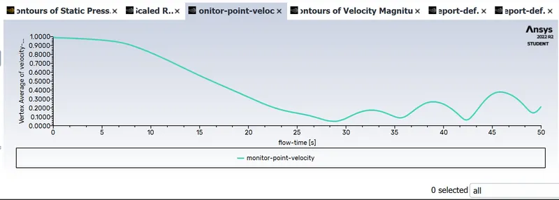
Monitor point velocity = 0.312 m/s
Velocity Contour
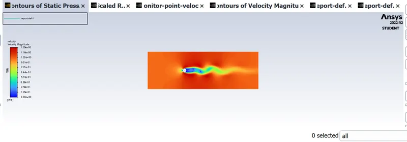
In the above diagram we can see the Von Karman vortex that appeared at around 300th time step and the process is called vortex shedding
Pressure Contour
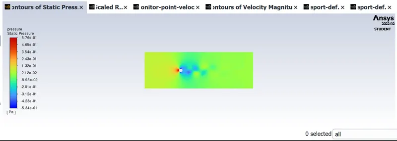
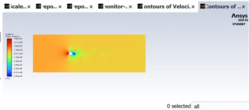
In pressure contour image, the low pressure field is changling alternately. It can be seen by observing the blue area. The low pressure wake field is the primary physics to observe for this challenge.
Coefficient Drag
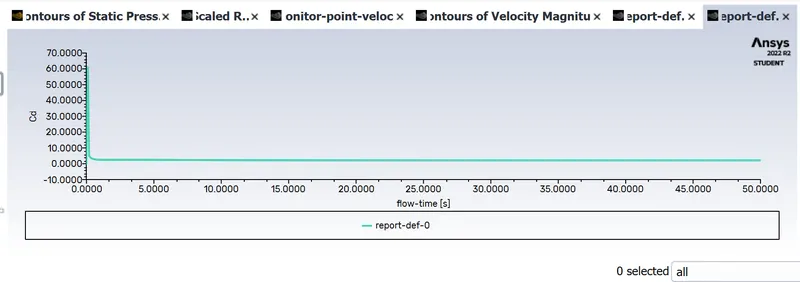
Coefficient of Drag = 1.416
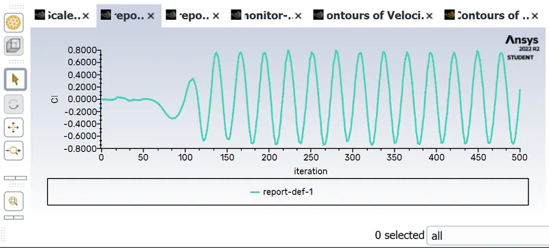
Coefficient of Lift
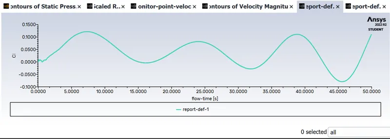
Coefficient of Lift = 0.101
STROHAUL NUMBER:
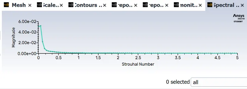
The strouhal number determined by taking the median of the plot data in the Fluent software is 0.25 for both steady & unsteady state simulation. Through analytical method, the strouhal number is calculated as 0.16. So, the strouhal number of fluent is nearer to the analytical method.
|
Solver |
Coefficient of Drag |
Coefficient of Lift |
|
Steady State Solver |
1.51 |
0.2613 |
|
Unsteady State solver (SIMPLE Method) |
1.41 |
0.101 |
PART 2
Under Steady state Condition at Re = 10, Viscosity = 0.02 kg/m sec, velocity = 0.1 m/s, Diameter = 2 Number of iterations = 500 iterations
Here we use the equation `Re = (rho*v*d)/nu`.where rho =1, d =2 , nu = 0.02 at Re = 10
v = 0.1 m/s
Residuals
MONITOR POINT VELOCITY:
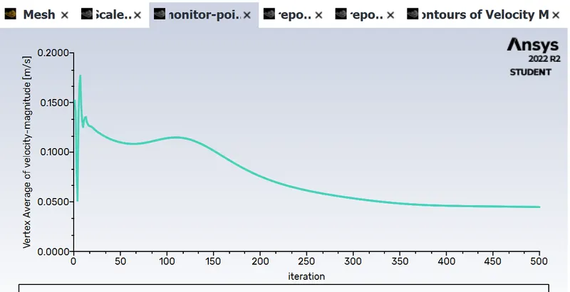
Average velocity = 0.0466
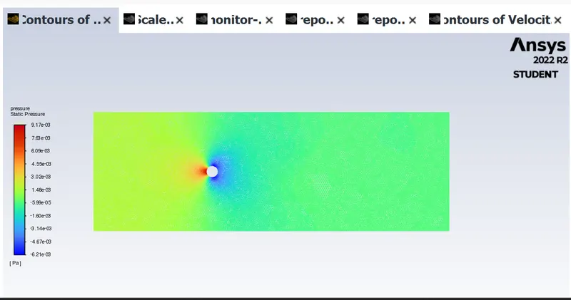
Velocity Contour
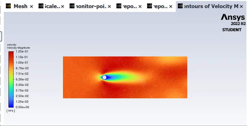
Pressure Contour
Coefficient Drag
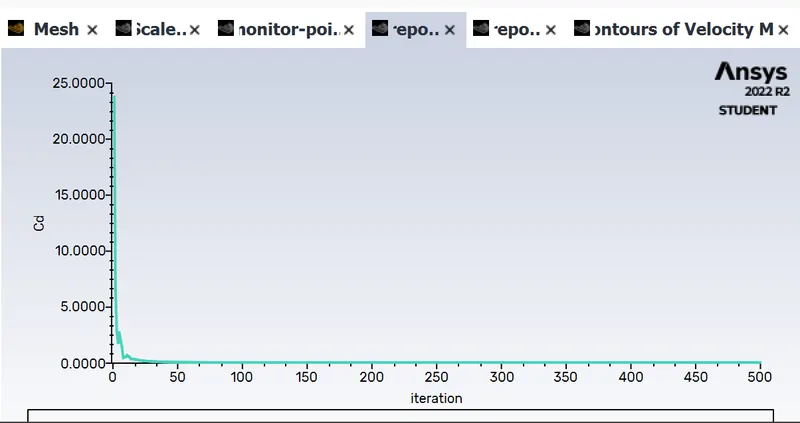
Coefficient Drag = 1.81
Coefficient of Lift
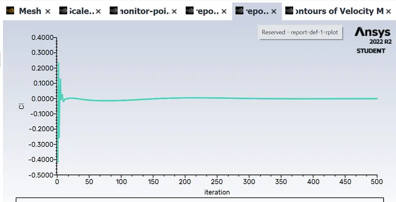
Coefficient of lift = 0.0088
Re = 100
v = 1 m/s
Residuals
This plot helps in monitoring the change in each and every convergence criterion for every time step and plots those values for every iteration or time step. This plot helps to know when convergence is achieved.
From the above plot, we can see that the solution has reached a steady state even before 500 iterations.
MONITOR POINT VELOCITY:
The average velocity is approximately 0.6 m/s
Velocity Contour
Pressure Contour
Coefficient Drag
Coefficient of drag = 1.5105
Coefficient of Lift
Coefficient of Lift = 0.2613
Re = 1000
v = 10 m/s
Residuals
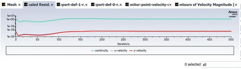
MONITOR POINT VELOCITY:
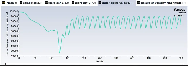
The average velocity is approximately 9.08 m/s
Velocity Contour
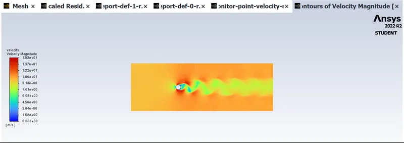
Pressure Contour
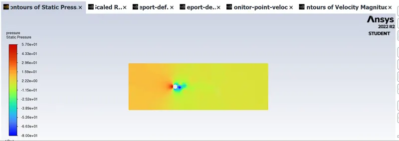
Coefficient of Drag
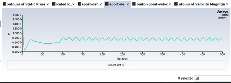
cd= 0.98
Coefficient of Lift
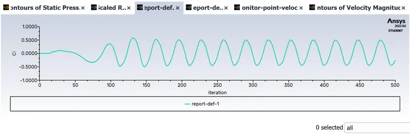
cl = 0.52
Re = 10000
v = 100 m/s
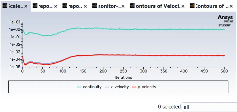
Residuals
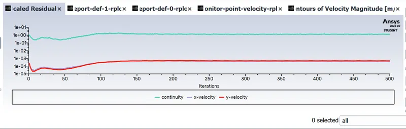
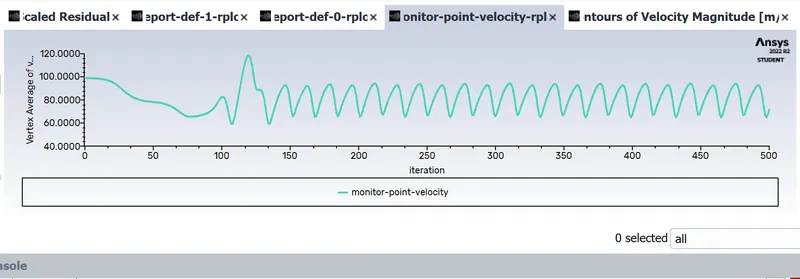
MONITOR POINT VELOCITY:
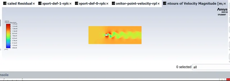
Velocity Contour
Pressure Contour
Coefficient of Drag
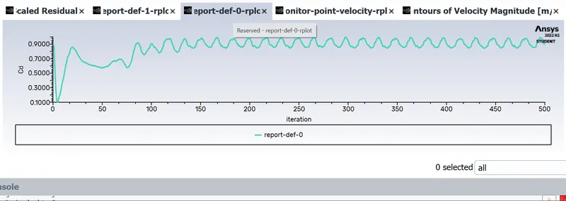
Drag Coefficient = 0.81
Coefficient of Lift
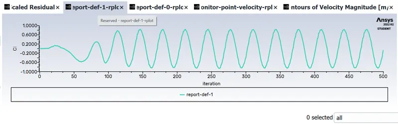
Lift Coefficient = 0.63
Re =100000
v = 1000 m/s
Residuals
MONITOR POINT VELOCITY:
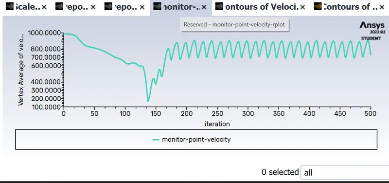
Velocity Contour
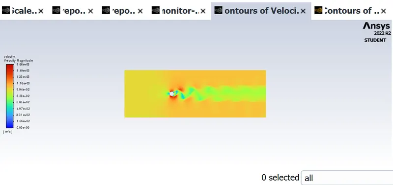
Pressure Contour
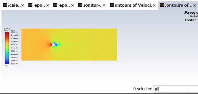
Coefficient of Drag
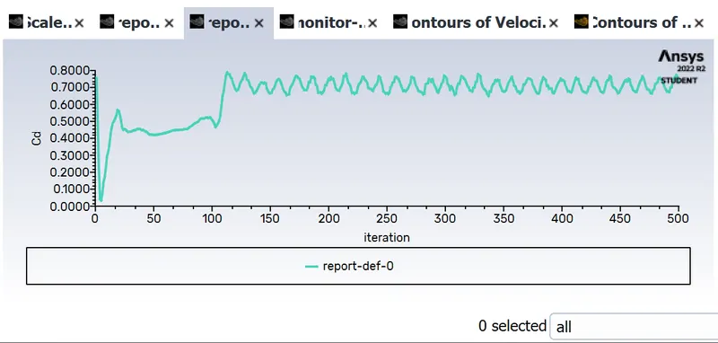
Coefficient of Drag = 0.71
Coefficient of Lift
Coefficient of Lift = 0.78
Comparison Table of Reynold number with Coefficient of Drag & Lift
| Reynolds Number | Coefficient of Drag | Coefficient of Lift |
| 10 | 1.81 | 0.00808 |
| 100 | 1.51 | 0.26 |
| 1000 | 0.98 | 0.51 |
| 10000 | 0.81 | 0.63 |
| 100000 | 0.71 | 0.78 |
CONCLUSION
1) If we compare the data in the table, it is seen that as Reynolds number is increasing the coefficient of Drag is decreasing and coefficient of lift is increasing. This data is compared with research paper given for reference and another research paper titled as "Simulation of Cross flow Induced Vibration" by Eric Williams et. al.
This phenomenon is happening because of when Reynolds number get increased the surface friction between fluid and cylinder is also increasing which casue the boundary layer to break before flow seperated hence amount of drag get decreases and lift get increases.
2) As the Reynolds number increase in value the wake region behind the cylinder is also increasing which results in bigger domain capturization for further simulations.
3) For lower Reynolds number the vortices are bit symmetrical in nature but as Reynolds number get increase it start to deviate more.
4) It can be seen that the steady state solver are more time friendly compared with transient one but Non-iterative Time Advance method can provide better opportunity to solve same trasient problem with less number iteration and time also.
REFERENCES
https://www.sciencedirect.com/science/article/pii/S0307904X08000243
Google and Wiki