Week 2 - Flow over a Cylinder.

Aim : Simulate the flow over a cylinder in ANSYS FLUENT to analyse the Von Karman vortex street.

introduction : Here the analysis of two-dimensional flow past a circular cylinder in different laminar flow regime is conducted. The analysis is done in ANSYS Fluent, the results of steady state unsteady (transient) state are anyalsyed . pressure based finite volume method is used for the time. accurate computation of incompressible flow. the effect of Von karman street is analysed using the reports og the analysis Various properties are plotted in order to find their relationship with the Reynolds number.

Procedure :

• Create the geometry in space claim
• In mesh, adjust the resolution of cylinder hole
• Create inflation layer originating from the outer boundary of the cylinder hole
• Mesh the geometry
• Name the sides
• Define fluid properties and boundary conditions
• Define Reynolds number
• Run the simulation in steady state and transient flow
• Analyse the results
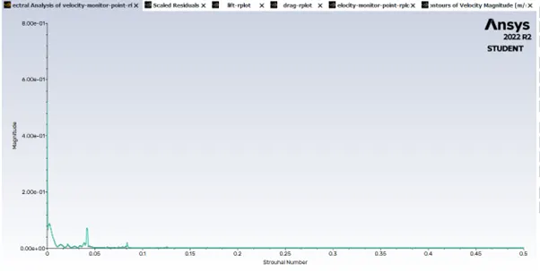
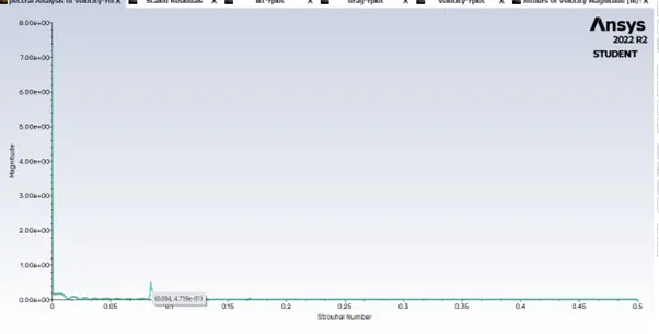
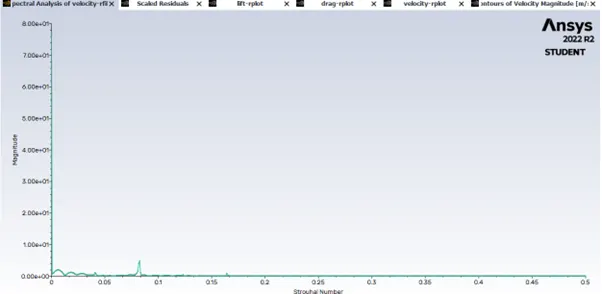
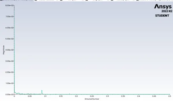
• Check the Strouhal’s number

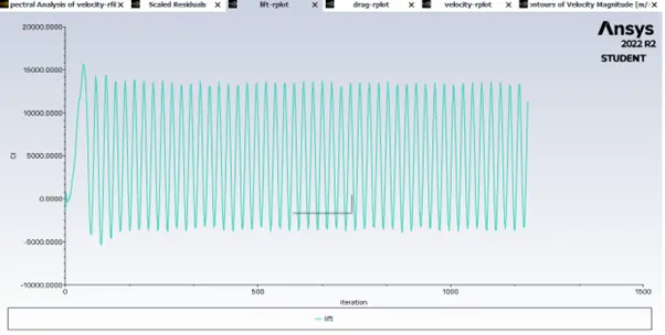
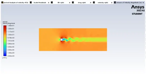
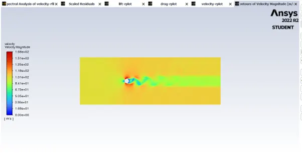
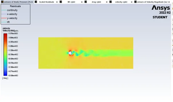
The simulation is done in Ansys fluent to analyse and understand the effects of von Karman vortex street. The von Karman vortex street is caused by a process known as vortex shedding; this causes the fluids to form an unsteady flow around blunt body. It creates a pattern of swirling vortices.

The formation of a vortex flow can only be seen in certain range of flow velocities specified by a rage of Reynolds number (Re).

Re= `frac{rho vd}{mu}`

`rho`= density

V = free stream velocity of fluid

D = diameter of pipe

`mu` = kinematic viscosity of flowing fluid

The Strouhal number represents the ratio of inertial forces due to the local acceleration of the flow to the inertial forces due to the convective acceleration.

St=`frac{fd}{u}`

f = frequency of oscillation

d = diameter of cylinder

u = velocity of fluid.

Designing of the computational fluid:

The model is created using ANSYS Space claim. teh diameter of the cylinder is considered to be 2 meters and the flow region is calculated using the centre of circle as initial point and diameter as reference length. The forward distance (outlet) is taken as 20D from the centre of circle and in teh backward direction (inlet) it is taken as 10D. above and below the distanc eis taken as 5D from centre. after creating the plane the pull tool used to create the surfaces surrounding the outer of the circle.

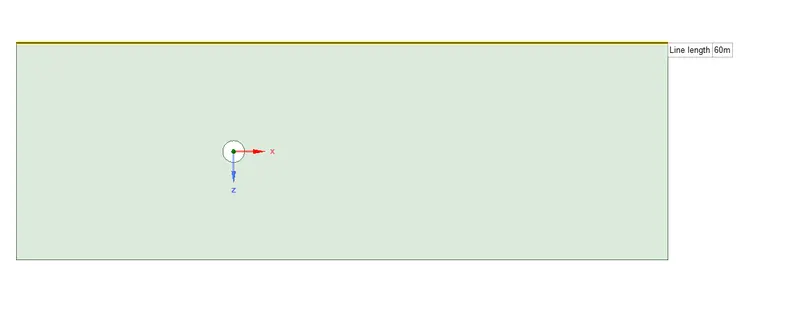
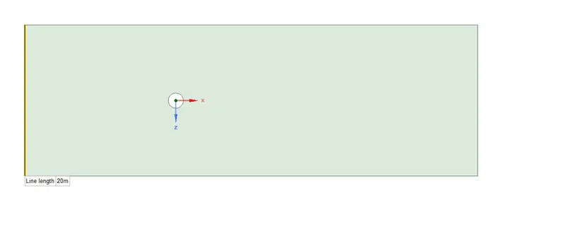
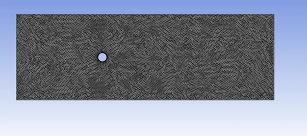
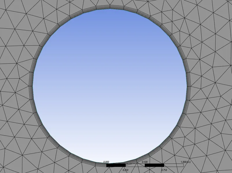
after that the mesh i sgenerated in ANSYS mesh. while creating mesh the inflatio layers are created from the outer of the circle to the outer symmetry walls. the mesh sizing is adjusted inorder to create a refined mesh. we require a refined mesh in ordere to obtain a proper result in th eanalysis. so the elements are meshed with a lenght of 0.25m. after meshing the sides afe named. the left side as inlet and right side as outlet. the boundary of the cylinder is named as walls and the top and bottom as symmetry . method was used ot set the mesh type to triangular. edge sizing is uded to get a proper geometry of teh cylinder and the hole defined per divisions and the number of divisions is set ot 36. 6 infation layers were created to get the proper values of velocity pressure and other parameters at the surface of th cylinder. the minimum tickness of teh inflatio layer was set to .005 with a growth rate of 1.2.

mesh > insert > method > geometry > method > triangles

mesh > insert > sizing > geometry > defintion type > number of divisions

mesh > insert > inflation > geometry >boundary > inflation option > first layer thickness > maximum number of layers

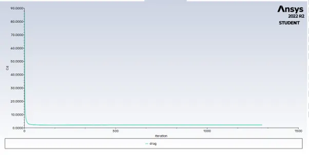
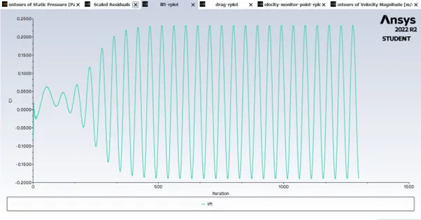
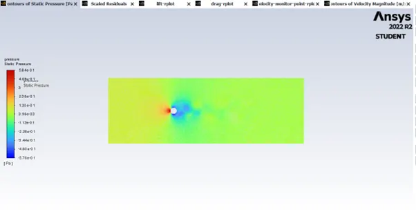
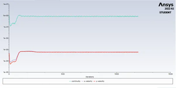
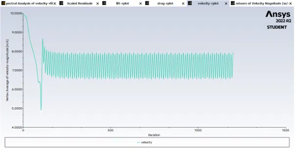
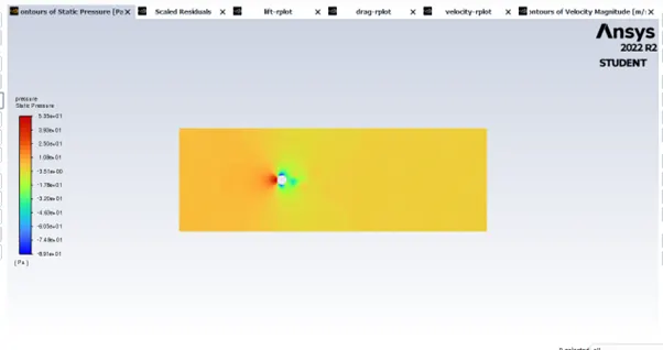
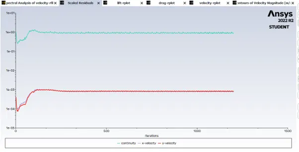
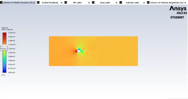
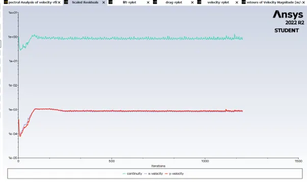
go to ANSYS fluent CFD solver use steady state pressure based solver. in results set monitoring point to analyse the results. in physics create a fluid of our own and set viscousity to 0.2 and density as 1. and in cell somes set material as new material and then in boundary condition set velocity to 1 so as to get the reynolds number of 100. in solutions definitions create a plot for vertex average at the monitor point. and in residuals remove the convergence criteria. define the coeficient of lift and drag. then initialize the hybrid initialisation. after intitialisation create a contour for the velocity and pressure. create a solution animationon velocity to check for vortex shedding. then run the iteration for 1200 iterations and check results. also repeat the process with a transient state solver adn analyze the result. check for vortex shedding in both cases. plot teh strouhal number suing the fft option for teh simulation to find out the strouhal number.

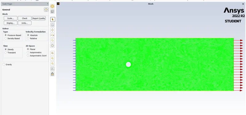
part 1

Case	Density	Velocity	Characteristic length	Viscosity	Reynolds number	solver	Drag coefficient	Lift coefficient
1	1	1	2	0.02	100	Steady state	2.177	0.136
2	1	1	2	0.02	100	Transient	2.23	0.479

case - 1 steady state solver

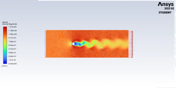
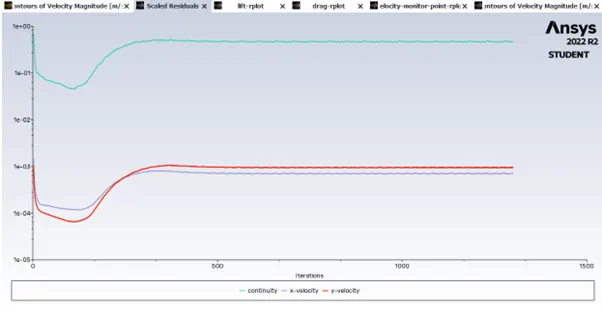
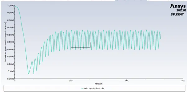
case 2 - transient solver

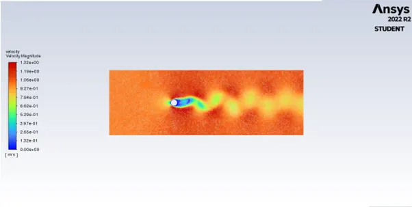
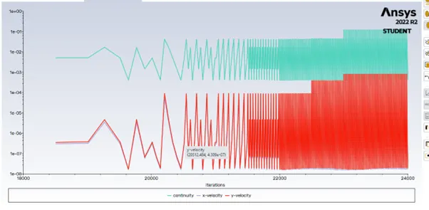
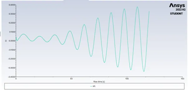
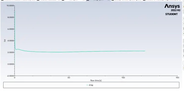
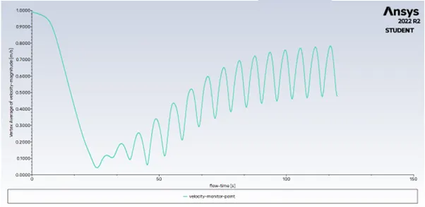
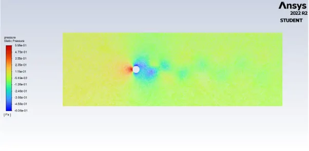
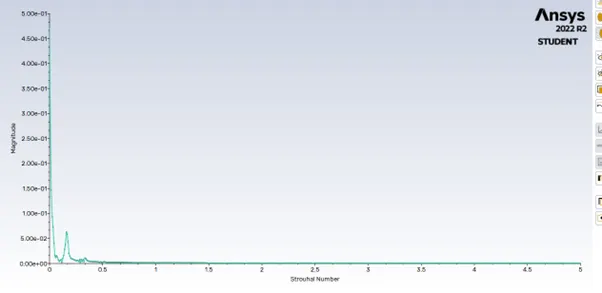
after runnig the simulation in transient state solver over a time frame of .1 and for 500 seconds the resulting strouhal number was compared with the reference values.

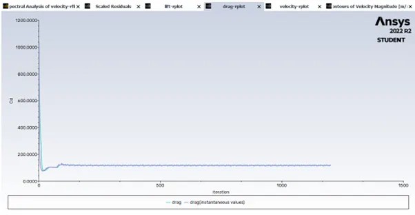
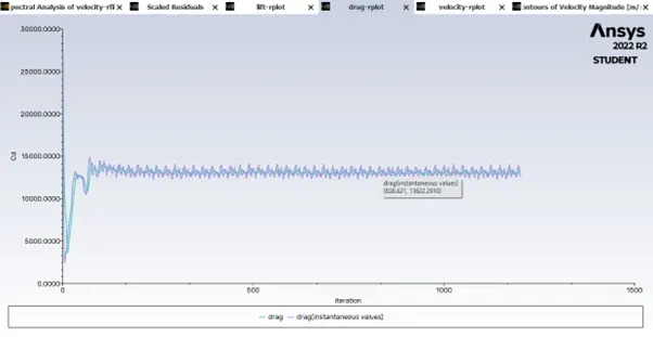
now to study the effec of reynolds number on the coefficient of drag the analysis is ina steady state solver with reynolds number 10,100,1000,10000 and 100000 and the results are also plotted. here the velociy is varied to anayle the effect o freynolds number on deag coefficient.

Part 2

Case	Density	Velocity	Characteristic length	Viscosity	Reynolds number	Drag coefficient (computed)
1	1	0.1	2	0.02	10	.054
2	1	1	2	0.02	100	2.177
3	1	10	2	0.02	1000	118.28
4	1	100	2	0.01	10000	12636
5	1	1000	2	0.002	100000	1352600.4

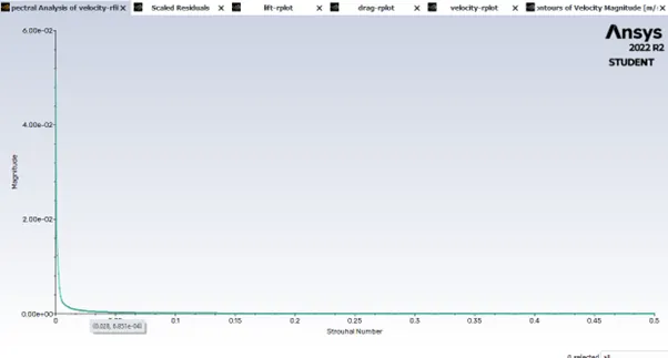
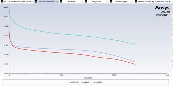
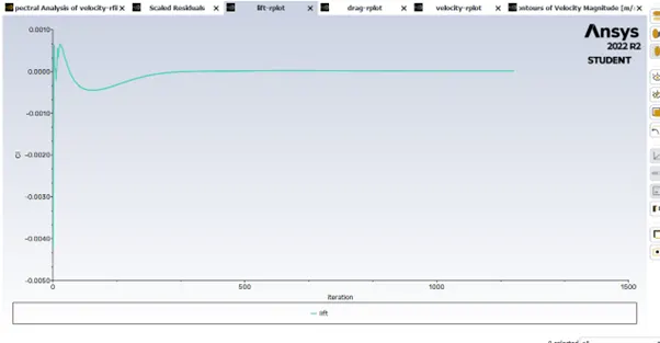
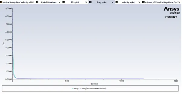
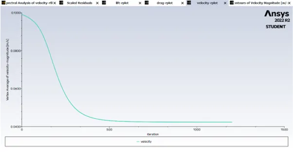
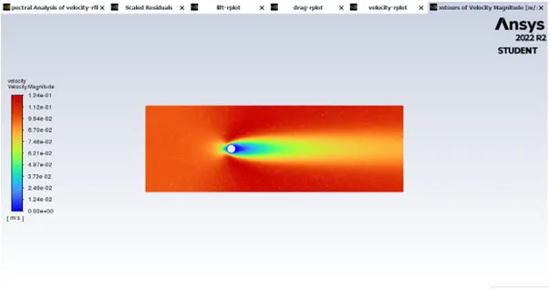
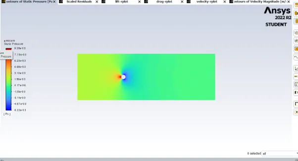
Reynolds number 10, case-1

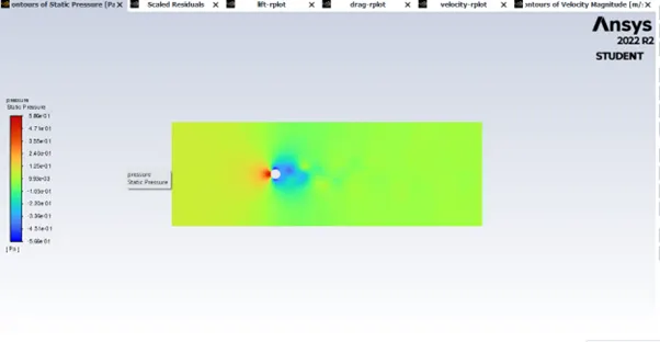
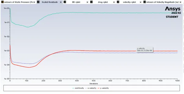
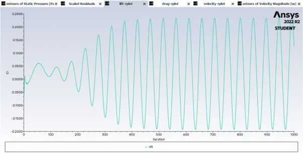
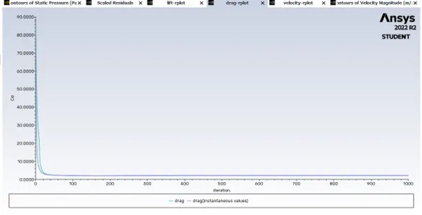
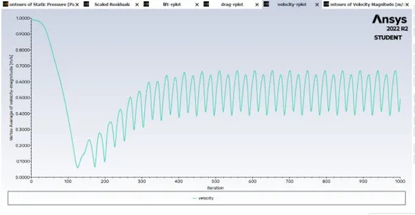
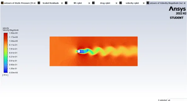
case-2, reynolds number 100

case-3, reynolds number 1000

case- 4, reynolds number 10000

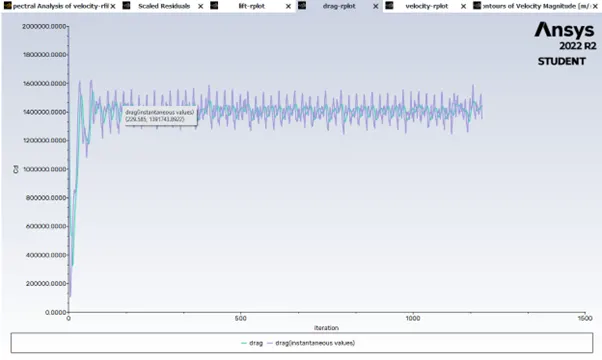
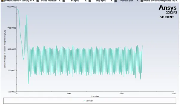
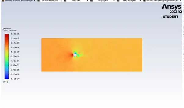
case-5, reynolds number 100000

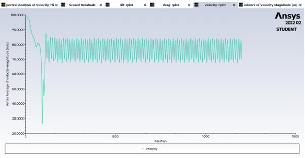
conclusion : from the analysis it was that when the reynolds number was 10 there was no vertex shedding happening but from Re of 100 we can see vertex sheddig happening. It was found that and the drag coefficient seems to exponentialy increase with increase in thereynolds number. The velocity of the flow semms to have an oscilatory effetct except for reynolds number of 10. and we were able ot see the boundary layer seperationn in the vertex flow. we can see that in vertex flow even wehn th eflow is having an oscilatory effect the variation of velocity in a repetetive cycle and we can say that teh flow can converged. when the Re was 10 the convergence can be easily identified as there was no oscilationns in the velocity of flow and the flow vertex reached a steady state after a few iterations.

Result. The analysis of flow of a liquid over a cylinder was simulated and the Von karman vortex street was also studied unervarious range of Reynolds number. the change inn coefficient of lift with respect to Reynolds number was also studied.