Flow over a cylinder

Aim : Simulate the flow over a cylinder and explain the phenomenon of Karman vortex street.

Objective :

PART-I

• Simulate the flow with the steady and unsteady case and calculate the Strouhal Number for   Re= 100. 

PART-II

1. Calculate the coefficient of drag and lift over a cylinder by setting the Reynolds number to 10,100,1000,10000 & 100000. (Run with steady solver)
2. Discuss the effect of Reynolds number on the coefficient of drag. [ Results should be validated with any standard literature and error should be within 5 %]

Expected results:-

1. In both approaches, show that the flow has converged. That is, what quantities or plots need to be looked at to determine that the flow has converged?
2. Plots of the coefficient of drag and lift. 
3. Plots to show vortex shedding behind the cylinder. 
4. Mention the referred material (Reference Paper or Fluid Mechanics Textbook) at the end of the challenge submission page. 

Theory :

1.     Reynolds number :

• The Reynolds number is a dimensionless number , named after the Osborne Reynolds , defined as the ratio of inertia forces to the viscous forces. Mathematically it is given as,

`Re="Inertia force(Fi)"/"Viscous force(Fv)"`

i.e.   Re=`(rhovD) / mu = (vD)/ nu`

where ,

ρ = density of fluid (kg/m³)

V = velocity of fluid (m/s)

D = diameter of pipe (m)

μ = dynamic viscosity of fluid (N-s/m²)

`nu` =  kinematic viscosity of fluid (m²/s)

• Significance :
  • Reynolds number is used in the forced convection. Forced convection is a type of heat transfer in which fluids are forced to move in order to increase the heat transfer.
  • Reynolds number is used to predict the flow patterns in the different fluid flow situation. At a low Reynolds number , the flow tends to be laminar flow, while at a high Reynolds number flow tends to be turbulent flow.

2.     Type of flow :

• Laminar flow :
  • If a fluid travels smoothly in a regular path then flow is called as laminar flow. if flow is to be called laminar flow when the following conditions satisfy.
  • For internal flow, Re < 2000.
  • For external flow, Re < 10⁵.
• Turbulent flow :

• If a fluid flows in a irregular path instead of regular path, then it is called as turbulent flow. The flow to be called as turbulent flow when following conditions occurred.
• For internal flow, Re>4000
• For external flow, Re > 5 x 10⁵.

3.     Lift and drag force :

1. When any body moves through a fluid , an intersection between the body and the fluid occurs and this effect can be described in terms of the forces at the fluid-body interface.
2. Both shear stress and pressure vary in magnitude and direction along the surface.
3. The resultant force in the direction of the upstream velocity is termed as Drag (D), and the resultant force normal to the upstream velocity is termed as Lift (L).

 

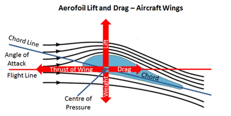
3.1.   Drag Force(Fd) :

• Drag force is a resistance forced which is acting opposite to the motion of the object.
• It is mathematically given as

Drag force(Fd) = `(underset(d)CrhoAV^2)/2`

Where ,

Cd = coefficient of drag

V = flow velocity

A = the projected area of the object  w.r.t.  which drag force is calculated.

 ρ = density of fluid

• Drag coefficient is a dimensionless quantity used to determine the drag or resistance of an object in a fluid environment such as air ,water.

3.2.  Lift force (F_l) :

• The force which is acting perpendicular to the object/body motion is called as lift force.
• It is mathematically given as

Lift force(Fl) =`(underset(l)CrhoAV^2)/2`

Where,

Cl = coefficient of lift.

• Lift coefficient is a dimensionless quantity which is used to determine the lift of an object in a fluid environment such as air , water.

4.     Flow separation :

• When a fluid is forced to flow over a curved surface at high velocities. A fluid follows the front portion of the curved surface with no problem but it has difficulty remain attached to the surface on the back side. At sufficiently high velocities, the fluid detaches itself from the surface of body. And this phenomenon is called as flow separation.
• The location of a separation point depends upon various factors such as Reynolds number, the surface roughness, the level of fluctuation in the free stream. And it is usually difficult to predict exactly where the separation will occurs unless there are sharp corners or abrupt changes in the shape of the solid surface.

                  

 

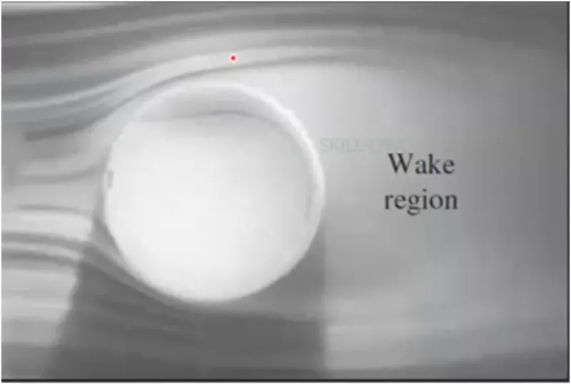
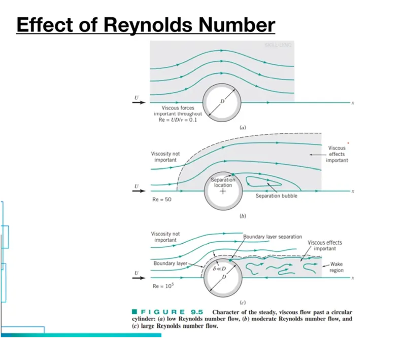
From above figure we can see that as Reynolds number increases the separation point moves towards left side and behind the cylinder wall the wake region increases.

5.     Von-Karman vortex street :

• When the fluid flows towards the body, the flow around a bluff body produces a regular patterns of alternating vortices known as Von-Karman vortex street. The following figure shows Karman vortices visible in the clouds.

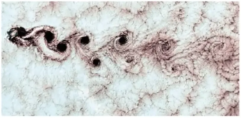
• These vortices produce a sinusoidal force acting on the body perpendicular to the flow. For a cylinder, the frequency (`omega`in Hz) of the shedding is related to the diameter(D in m) and wind speed (V in m/s) given by Strouhal number(S)

S =`(omegaD)/V`

• Strouhal number (St) :

• In dimensional analysis, the Strouhal number (St) is a dimensionless number describing oscillating flow mechanisms.

6.     Boundary layer concept :

• When any viscous flow flows over a surface, a region of slow-moving flow called boundary layer develops.
• Inside the boundary layer, there is a strong velocity gradient and U varies non-linearly.

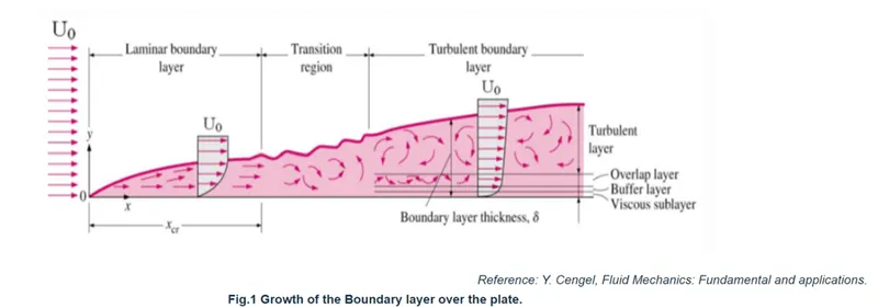
• The boundary layer comprises of –
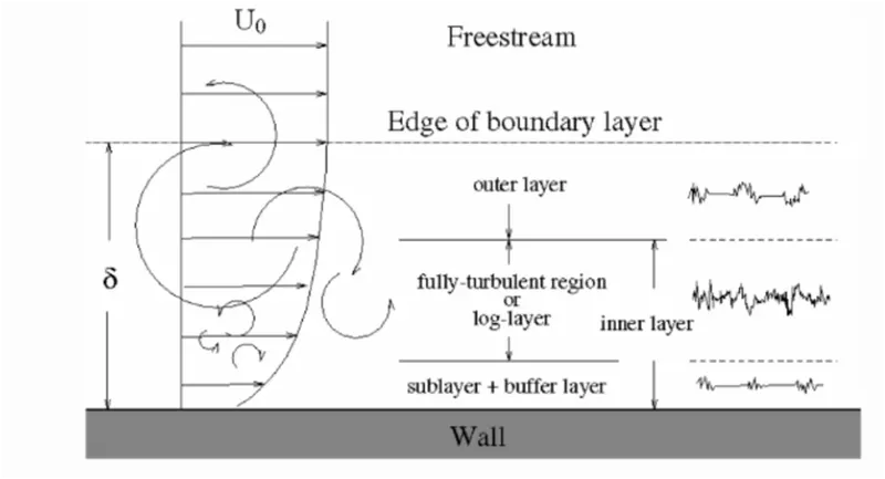
  • Inner layer i.e. 10-20% of total boundary layer thickness
  • Laminar sub-layer closest to the wall where viscous force dominates
  • Buffer layer where viscous and turbulent forces are of similar magnitude.
  • Log-law layer where turbulent forces dominates and velocity exhibits logarithmic variation.
  • Outer layer (law of the wake) where inertia forces dominates and flow is free from viscous effects.

7.     Y-plus :

• The behaviour of the flow near to the wall is a complicated phenomenon and to distinguish the different regions near the wall the concept of wall has been formulated and this concept is called as y-plus. Thus it is a dimensionless quantity and is measured in terms of viscous lengths.
• To resolve the effects near the wall i.e. the viscous sublayer, the size of the mesh size should be small and dense enough near the wall so that almost all the effects are captured. But in some cases, if the wall effects are negligible then there is an option of including semi-empirical formulae to bridge between the viscosity affected region and fully turbulent region , and in this case , the mesh need not be small or dense near the wall i.e. course mesh required.
• Considering the first case, i.e. near wall modelling it is well known that the small size mesh is required but the question arises that how much small size mesh required? Thus, here the concept y⁺ comes into picture and based upon the Y-plus value the first cell height can be calculated. The near wall region is meshed using calculated first cell height with gradual growth in the mesh so that the effects can be captured and avoids large mesh cell counts.
• The boundary layer components can be distinguished as follows
  • Laminar sublayer : Y+ < 5
  • Buffer layer : 5< Y+ < 30
  • Log-law layer : 30 < Y+ < 300
• Some turbulent models resolve laminar sublayer while others model it. therefore it is important to place the first cell centroid in either laminar sublayer or lag-law layer acoordingly.
• For a CFD simulation, we can compute the first layer height for a desired Y+ value as

`y=(y^+mu)/(rhounderset(**)(u))`

Where,

`underset(**)(u)=sqrt(underset(w)tau/rho)`

`underset(w)tau=1/2*underset(f)Crhounderset(oo)U^2`

`underset(f)C=0.0576Re^(-1/5)`

`Re=(rhounderset(oo)UL)/mu`

Where,

y= first cell height

μ= viscosity

ρ = density of fluid

u_* = frictional velocity

τ_w = wall shear stress

C_f = skin friction coefficient

U_∞ = free stream velocity

L = boundary sublayer thickness

8.     Inflation layers :

• To capture the viscous effects near the wall we need small mesh size. to resolve the gradients, the cells need to be smaller normal to the wall than along the wall.

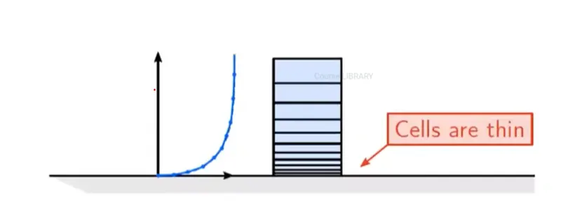
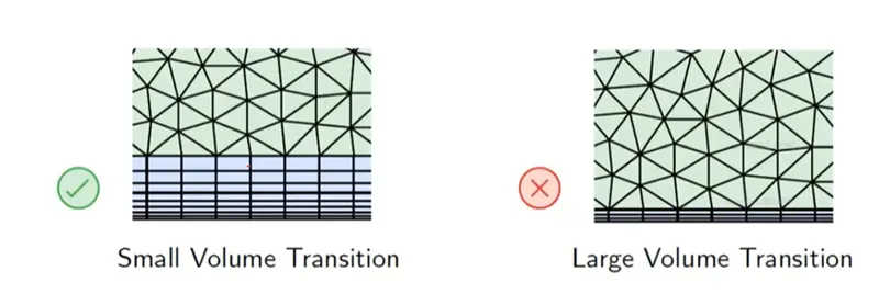
• Real geometries are complex and we often need to use an unstructured mesh. But the unstructured mesh are not thin enough close to the wall. so we can grow prism layers under beneath the unstructured mesh to provide the thin cells that we need to resolve the gradients. And these prism layers are called as inflation layers.

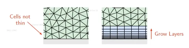
• It is common aim for the boundary layer thickness(δ₉₉) to be contained within the inflation layers. Hence, we need to formula to calculate the total height of the inflation layers. Then we can ensure that δ₉₉ is within the inflation layer.

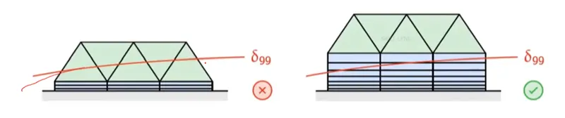
• There should be good volume transition required.

Procedure :

1.     Initial steps :

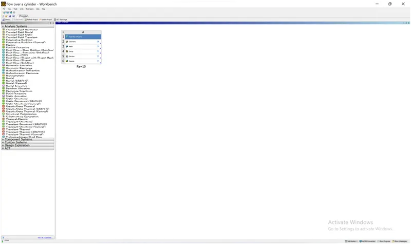
• Open the ansys workbench.
• Drag the ansys fluent model to the project schematic.

 

2.     Geometry :

• Right click on geometry and open spaceclaim.

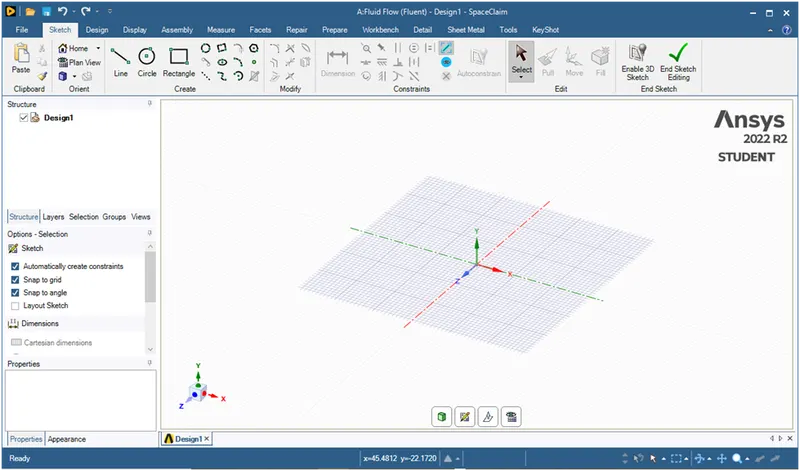
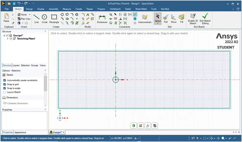
• Enable sketch mode.
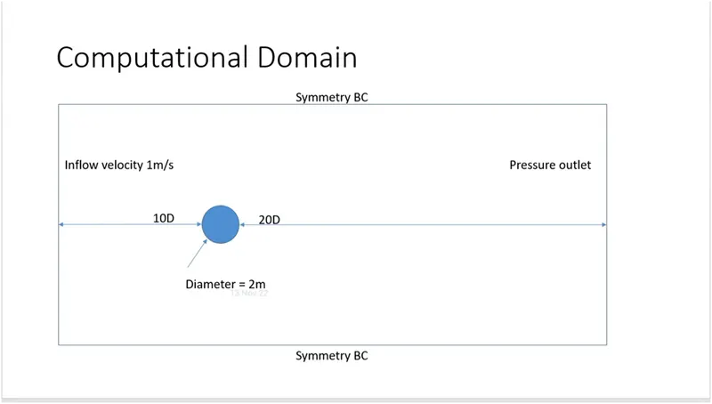
• Now we will create the computational domain as following dimensions

• After enabling sketch select xy-plane.
• Then create a circle of 2m diameter by using circle tool.
• Then create a construction line on left side of 20 m length from centre of circle and one more line in upward direction of 10m length.
• Then create a rectangle of dimensions 60m x 20 m by using rectangle tool.
• Then delete the construction lines by simply selecting lines and press delete key from keyboard.
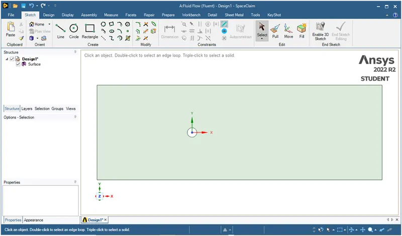
• Then use the pull tool for converting 1D geometry to 2D surface.
• After that delete the circle face to create a hole.
• The final geometry looks as

• After that close the space-claim.

3.     Mesh :

• Open the mesh

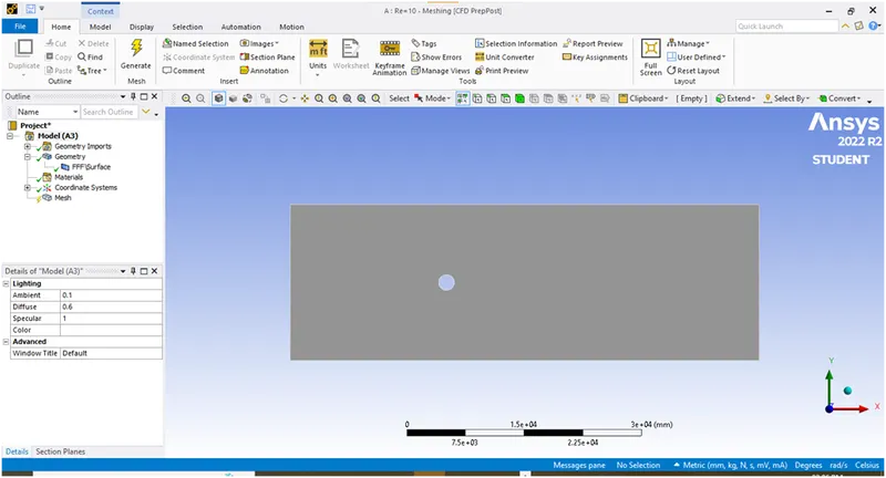
• Right click on mesh -> insert -> method -> select face -> apply -> select mesh method -> triangles
• Give mesh size=250 mm -> click on generate mesh.

 

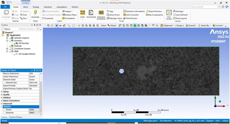
• After that to capture the boundary effects near the cylinder wall we have to create an inflation layer around cylindrical wall.for that right click on mesh -> insert -> inflation -> select face -> select boundary -> inflation option = first cell height -> size=5mm(we have calculated by using y-plus calculator online) -> no. of layers=20 -> right click on mesh and click on update.

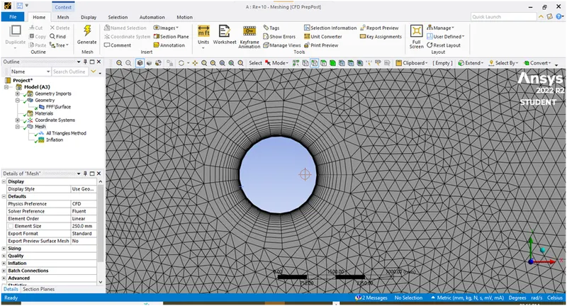
• We are not seen the good resolution of cylinder so to get good resolution insert the edge sizing method and give element size=100mm
• After that give the names to the geometry as inlet,outlet,cylindrical wall,symmetry as shown below

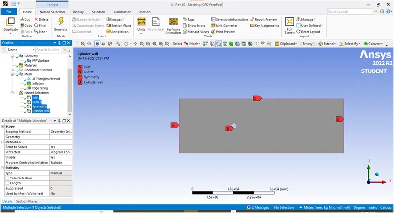
• After that just click on update and close this window.

4.     Post-processing methods :

4.1.           Setup :

• Open setup -> select double precision -> solver processors = 4 -> start

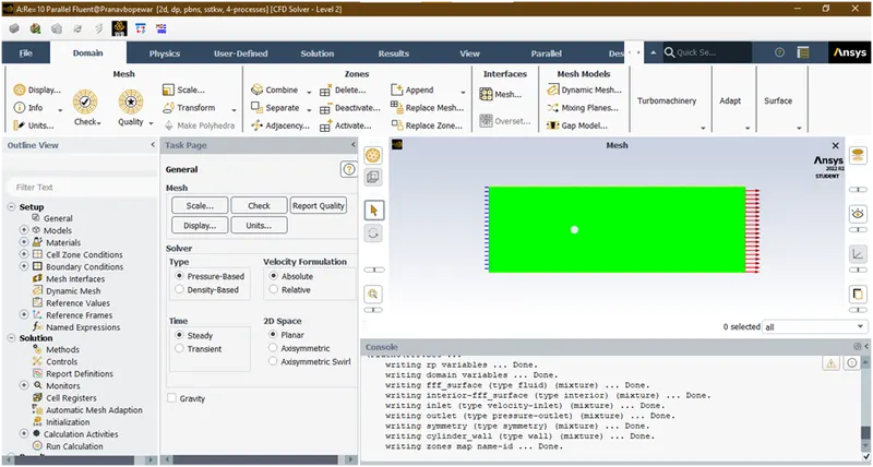
• Goto generals -> select pressure based type and steady state time
• Goto models -> viscous model -> laminar
• Goto materials -> fluid -> give density=1 kg/m3 , viscosity=0.05 pa-s
• Goto cell zone and apply this material.
• Goto boundaries -> inlet -> give velocity values as per required. i.e. for Re=10 V=0.25,for Re=100 V=2.5m/s etc.
• Change the reference values as length=2,area=2 and also cross-check other parameters.
• Goto Solutions -> methods -> Scheme -> simple
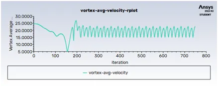
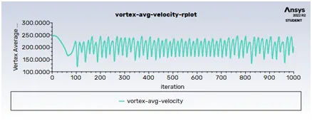
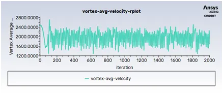
• Goto Solutions -> report definations -> create new reports as ->force-> drag , lift @ cylinder wall and new -> surface-> vortex avg-> velocity @ monitor point. To create monitor point behind the cylinder goto results -> right click on surfaces -> new  ->point -> x=4D=4x2=8,y=0
• Solutions -> monitors -> initialize -> hybrid initialize -> initialize for initializing the solution.
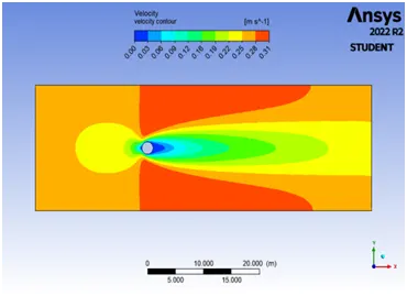
• Results -> graphics -> contours -> create velocity contour
• Solution -> run calculation for 1000 iterations to calculate all parameters which are required and to create the animation goto solutions-> activities-> create animation -> solution animation and select velocity contour as output then click on ok.
• now creates a velocity and pressure contours for different cases.to plots velocity and pressure contour goto results-> graphics -> contour -> and create contour which is required.
• Also compute drag coefficient , lift coefficient, vertex avg velocity at monitor point behind the cylinder wall.
• Plot strouhal no plot for Re=100 (steady and unsteady) and calculate for lift oscillations to plot strouhal number goto results -> plot -> fft -> select y-axis=magnitude, x-axis =st. number and load data file as lift file.-> then click on plot FFT.

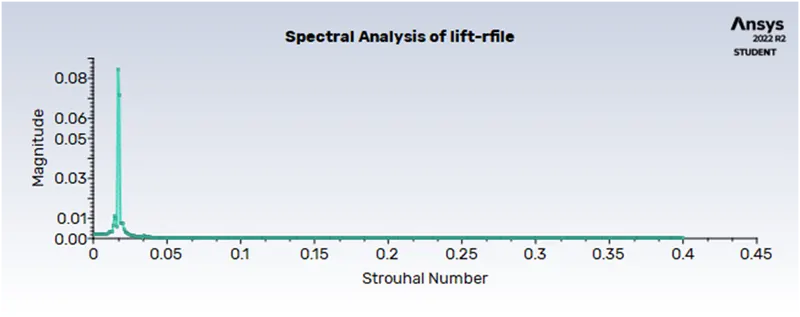
Fig : Strouhal number for Re=100(steady)

Now above figure we can see that the maximum samples are obtained for 0.086 magnitude so corresponding value from x-axis is our strouhal number for this case. And this is=0.017

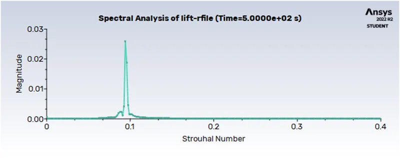
Fig : Strouhal number for Re=100(unsteady)

Similarly from above fig Max lift=0.0275 and corresponding St=0.095

Results :

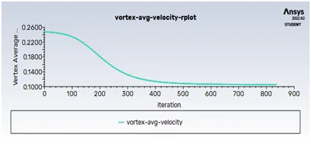
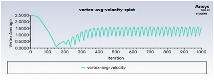
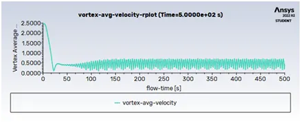
• Comparision of drag , lift coe. and vertex velocity for different cases and validation of values.

Cases	Velocity	Drag coe.	Lift coe.	Vortex avg velocity(m/s)	Strouhal number
Re=10(steady)	0.25	3.34	-0.00013	0.106	-
Re =100(steady)	2.5	1.48	-0.0023	1.23	0.017
Re=100(Unsteady)	2.5	1.291	-0.00064	0.52	0.095
Re=10^3(steady)	25	1.13	0.015	19.32	-
Re=10^4(steady)	250	1.275	-0.044	203.57	-
Re=10^5(steady)	2500	1.23	-0.0188	1975.15	-

 

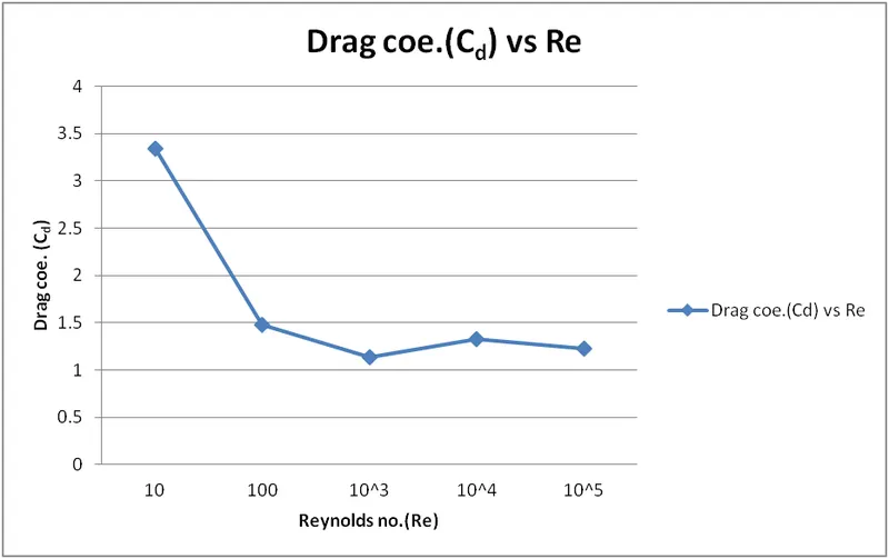
Figure 1

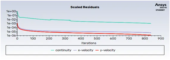
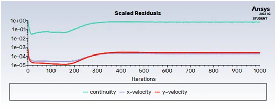
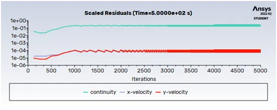
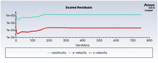
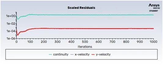
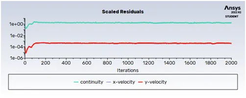
• Scaled residual plots

Cases	Residual plots
Re=10(steady)
Re =100(steady)
Re=100(Unsteady)
Re=1000(steady)
Re=10^4(steady)
Re=10^5(steady)

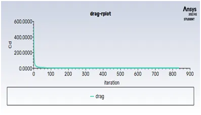
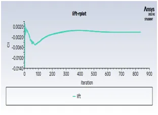
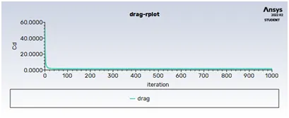
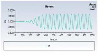
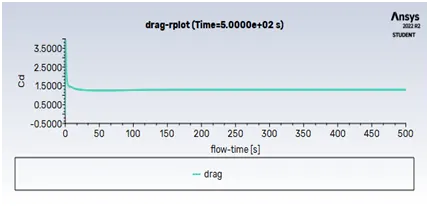
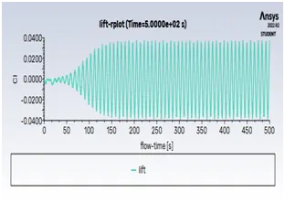
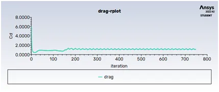
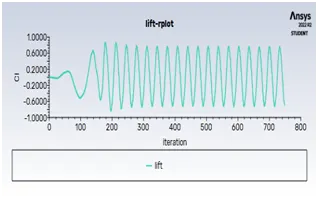
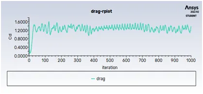
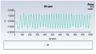
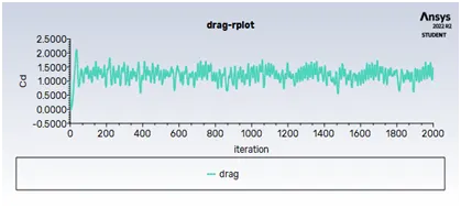
• Drag coe. , lift coe. plots

Cases	Drag coe. plot	Lift coe. plot
Re=10(steady)
Re =100(steady)
Re=100(Unsteady)
Re=10^3(steady)
Re=10^4(steady)
Re=10^5(steady)

• Plots to show vertex shading velocity behind the cylinder wall

Cases	Vortex avg velocity
Re=10(steady)
Re =100(steady)
Re=100(Unsteady)
Re=10^3(steady)
Re=10^4(steady)
Re=10^5(steady)

• Velocity and pressure contour plots

Cases	Velocity contour	Pressure contour
Re=10(steady)
Re =100(steady)
Re=100(Unsteady)
Re=10^3(steady)
Re=10^4(steady)
Re=10^5(steady)

• Animations

Cases	Gif files
Re=10(steady)
Re=100 (steady)
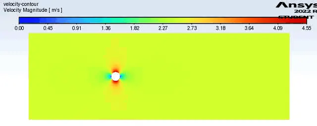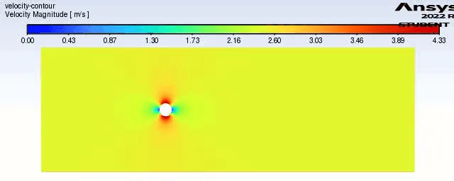
Re=100(Unsteady)

 

Conclusions :

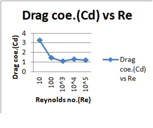
• Validation of drag coe.

Actual plot	Reference plot

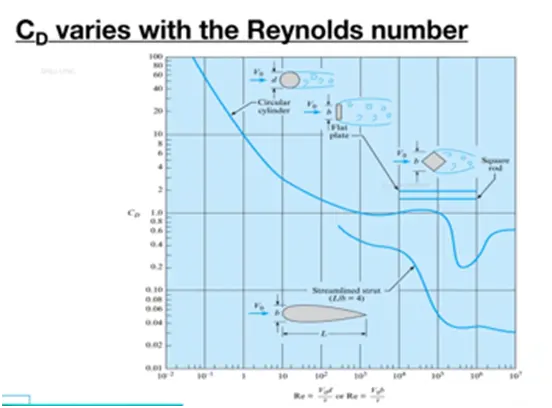By comparing these plots we can say that our results are matches with reference it means our values are validates.

• From residual plots we can say that the solution has been converged.here the convergence meaning after certain iterations the values of continuity,x-velocity,y-velocity are constant i.e. there is no change.
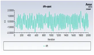
• From drag and lift plots we can say that for Re=10 the drag and lift coe. is not change that much and it can be found as mention in above result tables. But from Re=10 we are getting lift plots as oscillatory waves.it means that there is a vortex shedding has started. In this oscilaattory wave plot we can say that the plot get converge only when the amolitude of wave gets uniform. And we are computing the lift coe. as taking mean of these oscillatory waves. Also in vertex shadding velocity behind the cylinder gets as in wave forms so we are find out the velocity by taking mean of these oscilattory waves. And these all drag coe., lift coe., and vertex avg velocity compute and shown in table.
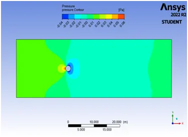
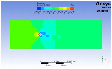
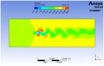
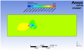
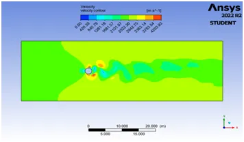
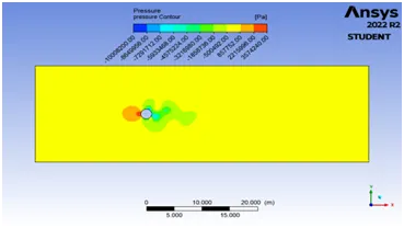
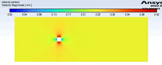
• From velocity contour for Re=10 we can say that the blue region show less velocity means around 0m/s and this is called as wake region and the flow separation starts at the cylinder wall this is due to drag force and also due to boundary phenomenon. And also seen from pressure contour there is a low pressure area crates near the wall. At frontal side there is a red contour shows in pressure contour it means there is pressure increases due to high impact of high velocity and due to this kinetic energy converts into pressure energy and due to impact the velocity becomes zero.also from velocity contour we can see some red region shows it means there is increase in velocity due flow separation takes place and there is a transfer of energy.
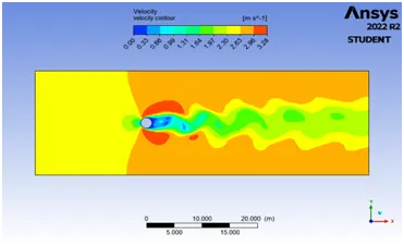
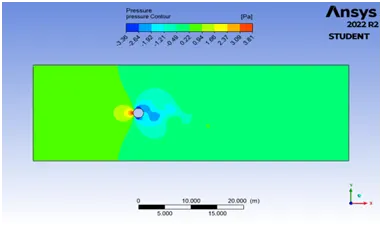
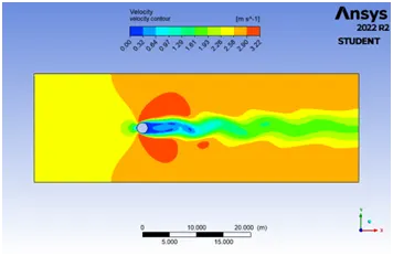
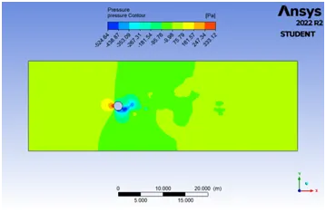
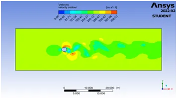
• For Re=100 we can see that behind the cylinder wall there is vortex shading started and there is reduction in wake region and separation point moves towards front side due to high velocity.and this results in increasing the pressure in frontal side. Now by comparing all velocity contours we can say that as velocity increases the flow separation points moves towards frontal portion and wake region decreases. And pressure gets uniform thoughtout the fluid domain.
• Also as Reynolds number increases the drag coe. reduces.
• Reference paper :  https://www.sciencedirect.com/science/article/pii/S0307904X08000243