Week 2 - Flow over a Cylinder.

AIM -

A simulation for external flow over a cylinder is to be performed using Ansys Fluent.

INTRODUCTION & THEORY -

• Types of Flows -

1. Laminar flow: If a Fluid travels smoothly in a regular path then it is called a Laminar flow.
2. Turbulent Flow: If a Fluid flows in an irregular path instead of a regular path, then it is called a Turbulent flow.

Flow Type	Value of Reynolds Number (Re)
	Laminar Flow	Transitional Flow	Turbulent Flow
Internal Flow	Re < 2300	2300 < Re < 4000	Re > 4000
External Flow	Re < 1 x 105	1 x 105 < Re < 5 x 105	Re > 5 x 105

• Karman Vortex Street -

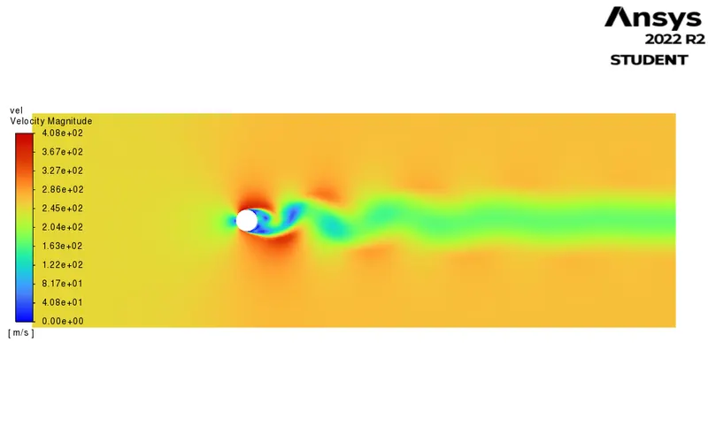
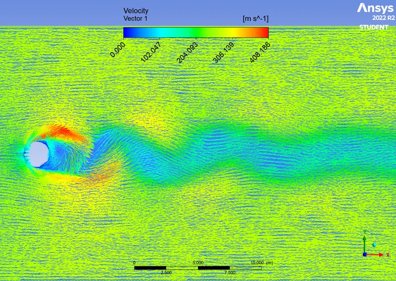
When the fluid flows towards the body, the flow around a bluff body produces a regular pattern of alternating vortices known as the "Karman vortex street".

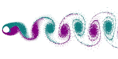These vortices produce a sinusoidal force acting on the body perpendicular to the flow. For a cylinder, the frequency (in Hz) of the shedding is related to the diameter `D` (m) and wind speed `v` (m/s) via the Strouhal number `S` such that `S = frac{omegaD}{v}` that is, the Strouhal Number is used to find the frequency of oscillation.

The Strouhal Number is a dimensionless value useful for analyzing oscillating unsteady fluid flow dynamics problems.

• Steady-state and Transient state -

The term "steady state" refers to a condition where a flow is balanced throughout the entire system and does not change over time. On the other hand, a transient state is an unbalanced state that changes over time.

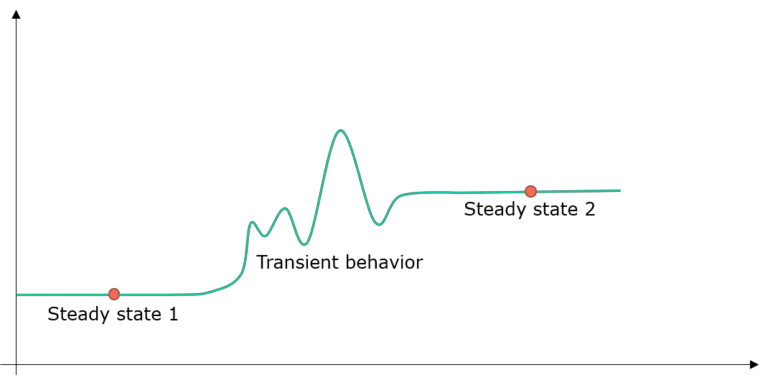All of the properties and flow conditions of the system are assumed to be constant over time in steady-state models. Transient models, on the other hand, can handle dynamically changing conditions and evaluate the effect of time on thermal and flow predictions. A straightforward example—taking a shower—can be used to demonstrate the differences between transient and steady-state calculations. A steady state simulation will only produce the shower water's temperature and flow rate, given the faucet's characteristics, the hose's dimensions, the inlet, and ambient temperatures. Additionally, even if you adjust the valves during warm-up, a transient simulation will show you how long it takes for the shower temperature to be comfortable.

• Drag and Lift -

When a fluid passes through an object or an object flows through a stationary fluid, the fluid exerts a force on the Object. This force has two components the one which acts in the direction of fluid flow is called 'Drag' and the other that acts in the direction perpendicular to the flow direction is called 'Lift'.

Drag Force:

Drag force is a resistance force which is acting opposite towards the motion of the object.

`F_D = frac{C_DxxrhoxxAxxV^2}{2}`

where,

`C_D` - Coefficient of drag

`V` - Velocity

`A` - Area

`rho` - Density

Lift Force:

The force which is acting perpendicular to the object/body motion is called Lift force.

`F_L = frac{C_LxxrhoxxAxxV^2}{2}`

where,

`C_L` - Coefficient of lift

`V` - Velocity

`A` - Area

`rho` - Density

SOLVING & MODELLING APPROACH -

With each CFD simulation, the following workflow is followed;

1) Problem finding
2) Pre-processing
3) Processor or Solver
4) Post-processing

A computational domain for the external flow analysis and a two-dimensional geometry model was created in SpaceClaim. Later, in the Mesh file, the appropriate mesh was created over the entire geometry & Named Selection was accomplished. The simulation was run for eight different cases in accordance with the conditions mentioned in the problem statement after the applicable solver settings were entered in the Setup file.

It is asked to run the simulation with the Reynolds numbers set to 10,100,1000,10000, and 100000 in the problem statement. The inlet flow's velocity must be changed in order to change the Reynolds number.

We know that, `Re = frac{rhoVD}{mu}`
where `rho` = Density of fluid (for air, `rho` = 1 kg/m³)
`V` = velocity of inlet flow,
`D` = characteristic length of flow (in this case, the diameter of the cylinder, `D` = 2 m)
`mu` = viscosity of fluid (for air, `mu` = 0.05 Ns/m²)

Case No.	Reynolds No. (Re)	Inlet velocity [m/s]	Solver Time
1	10	0.25	Steady
2	100	2.5
3	1000	25
4	10000	250
5	100000	2500
6	100	2.5	Transient
7	10000	250
8	100000	2500

During the post-processing phase, results were calculated and saved in the Result file as plots and contours. Conclusions were reached after evaluating the study results.

PRE-PROCESSING -

In SpaceClaim, first, change the unit system from millimetres to metres in the File menu. In the 'Sketch' mode, enable the XY axis and create a circle at the origin of the plane with a diameter (D) of 2 metres using the Circle command.

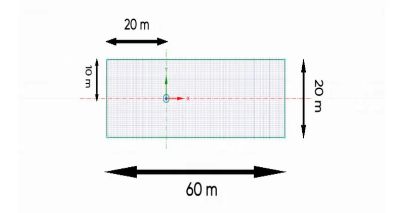
Now, in order to create a computational domain, we need to follow some parameters which are;

• The distance between the inlet of the computational domain and the centre of the cylinder should be 10 times the diameter of the cylinder (`10 xx 2 = 20` metres)
• The distance between the outlet of the computational domain and the centre of the cylinder should be 20 times the diameter of the cylinder (`20 xx 2 = 40` metres)
• The distance between the top and the bottom of the computational domain and the centre of the cylinder should be 5 times the diameter of the cylinder each (`5 xx 2 = 10` metres)

As a result, a rectangle 60 metres long and 20 metres wide must be created around the cylinder. To construct this rectangle, first, create a 20-metre-long line from the centre of the cylinder and a 10-metre vertical line upwards from the end of this 20-metre line using the 'Construction Line' command. The above-mentioned rectangle was constructed using the 'Rectangle' command.

Use the '3D' or the 'Pull' command to convert these lines into 2D surfaces as required according to the problem statement. Only the outer surface of the cylinder is required for the asked simulation of the external flow analysis of this cylinder.

Thus, the required geometry, a two-dimensional model of a cylinder and a computational domain around it, was created successfully.

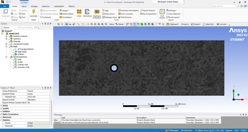
In the 'Mesh' file, generate the mesh over the model with the following information:

Baseline Mesh	Computational Domain	Cylinder Edges	Inflation Layers
250 mm	All Triangular Method	No. of Divisions = 72	Geometry: Computational Domain Boundary: Cylinder Edge
			First Layer Thickness = 5 mm Maximum Layers = 20 Growth Factor = 1.2

Note: Here, for inflation layers, we haven't used any external calculator to calculate the 'First Layer Thickness' as the geometry model is very simple and not very significant. Hence, assuming the model as simple geometry, the first layer thickness was taken as 5mm.

Named Selection:

Sr. No.	Component	Name Assigned
1	Inlet (Left) Edge of Domain	Inlet
2	Outlet (Right) Edge of Domain	Outlet
3	Cylinder Edge	Cylinder Wall
4	Top & Bottom Edges of Domain	Symmetry Wall

SOLVER -

In the 'Setup' file, provide the following solver settings:

Fluent Setup
Sr. No.	Setup	Command
1	Model	Laminar
2	Solver Type	Pressure based
3	Solver Time	Steady – Case 1 to Case 5
		Transient – Case 6 to Case 8
4	Energy	OFF
5	Material	Fluid – Air (Density = 1 kg/m³, Viscosity = 0.05 Ns/m²)
6	Reference Values	Compute from - Inlet
		In the Reference values, we must change the area, length, velocity, density, and viscosity with respect to our case
7	Inlet	Velocity Inlet
8	Outlet	Pressure Outlet
9	Method	SIMPLE

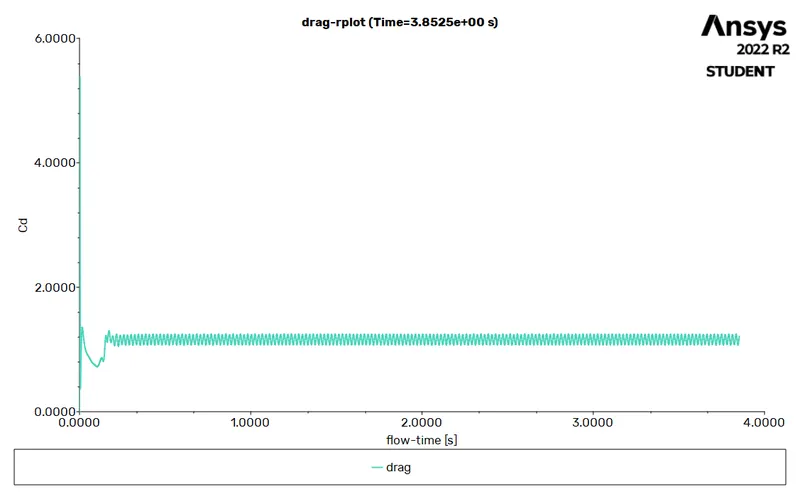
Since we need to determine the values of the drag and lift coefficients acting over the cylinder, a report was created using the 'Report Definitions' tool to calculate the drag and lift coefficients acting over the cylinder.

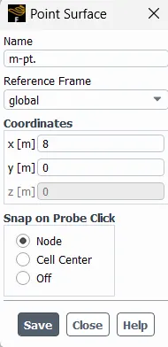
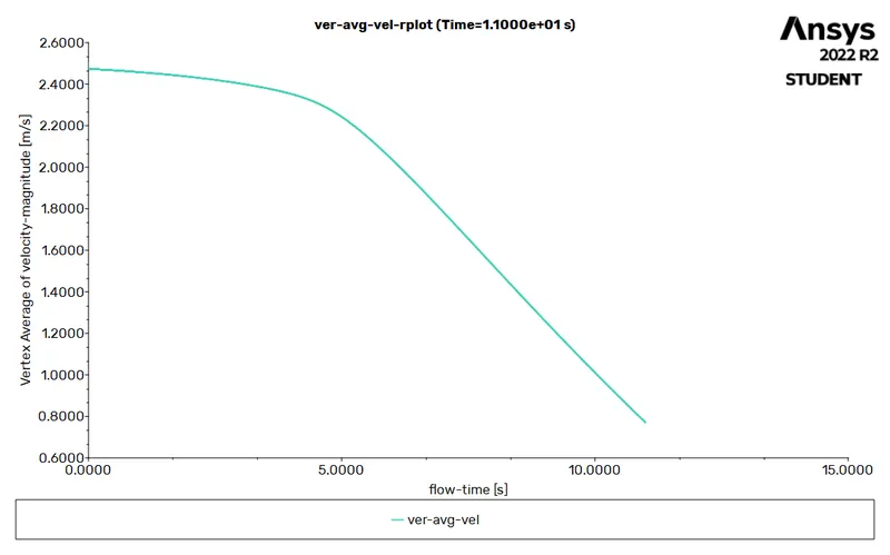
In addition, we will determine the flow's vertex average velocity at a point 8 metres from the cylinder's centre (in the positive "X" direction). The name of this point will be "Monitor Point."

Results > Surface > Create 'Point' > Name - Monitor Point > Coordinates - x = 8 m & y = 0 m > OK

We will now determine the vertex average velocity value, just as we did with the drag and lift coefficient plots.

Solution Toolbar > Definitions > New > Surface Report > Vertex Average > Name - 'vertex avg velocity' > Field Variables - Velocity & Velocity Magnitude > Surfaces - select the 'Monitor Point' > enable 'Print to Console' > OK

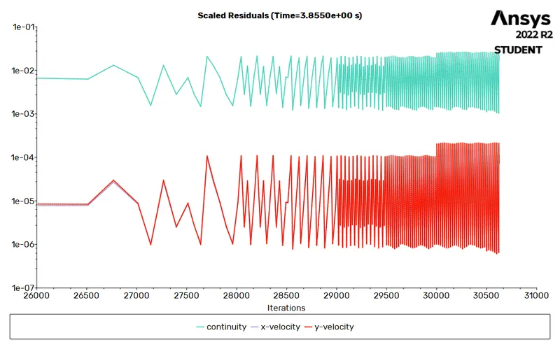
Initialize the solver settings and run the simulation for all cases for a specified number of iterations until convergence is reached.

Case No.	Plots
	Scaled Residuals	Drag Coefficient	Lift Coefficient	Vertex Average Velocity
1
2
3
4
5
6
7
8

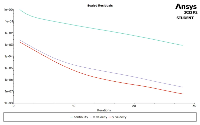
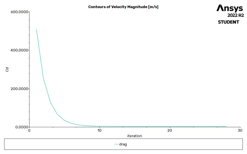
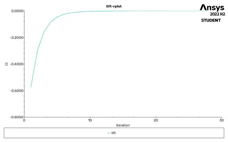
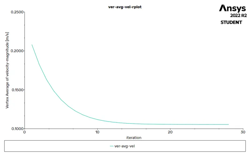
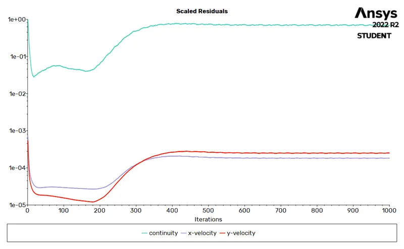
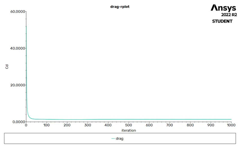
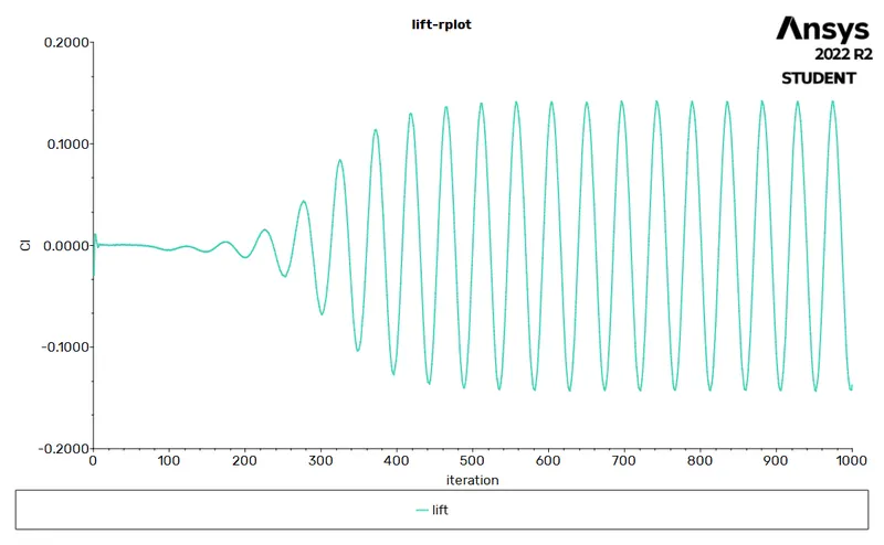
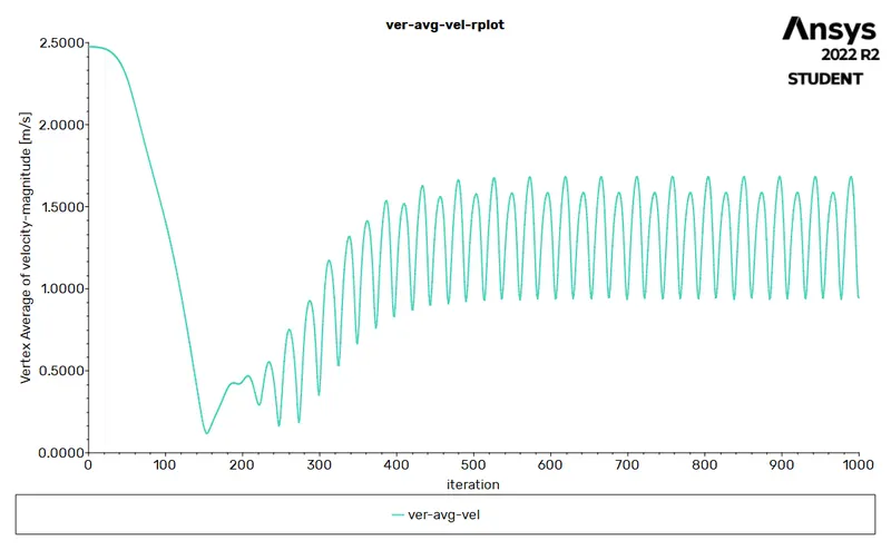
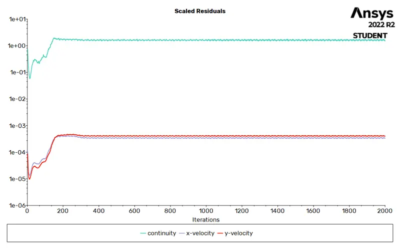
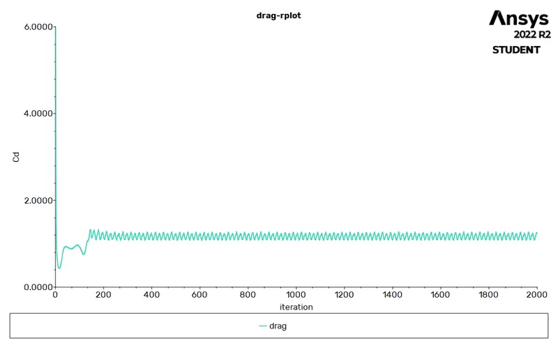
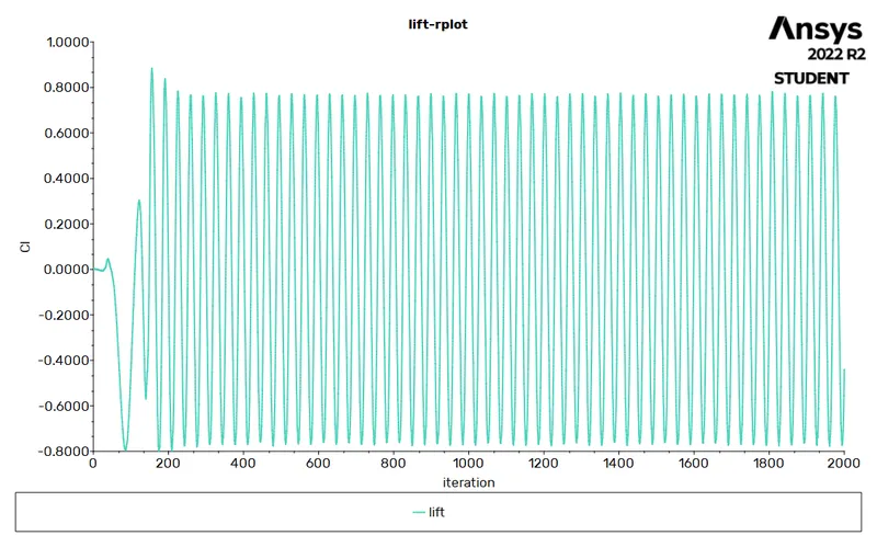
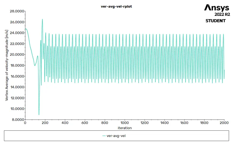
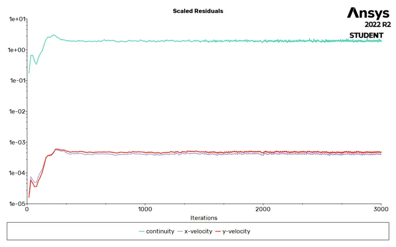
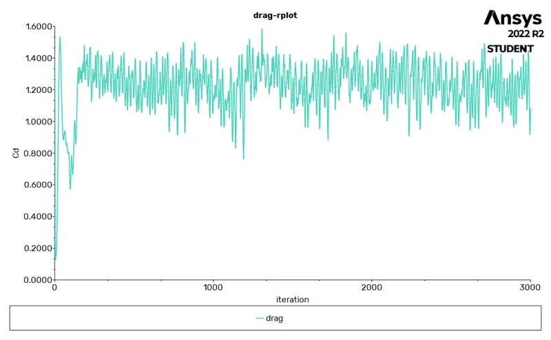
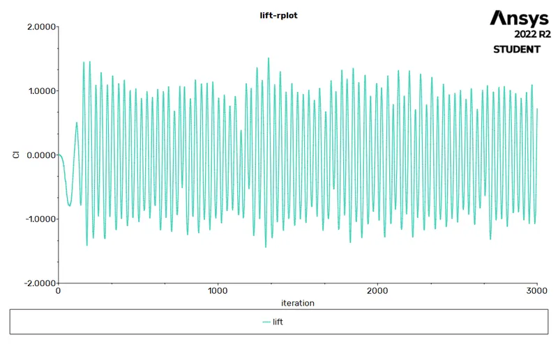
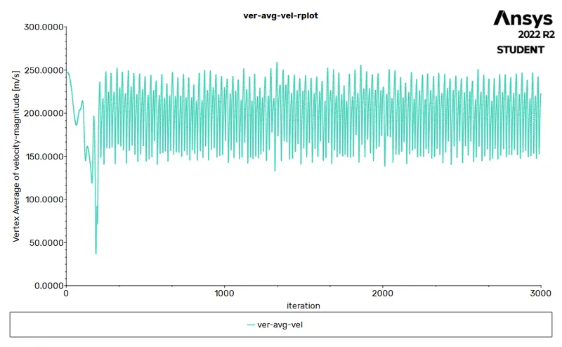
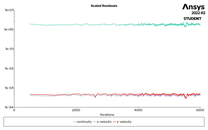
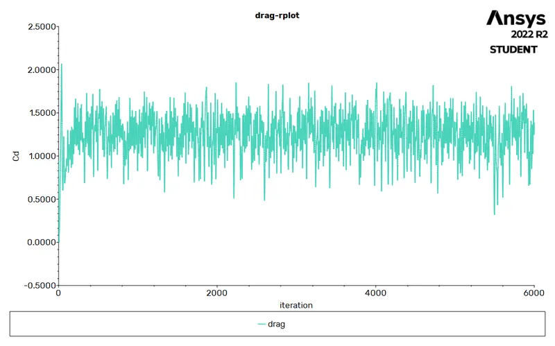
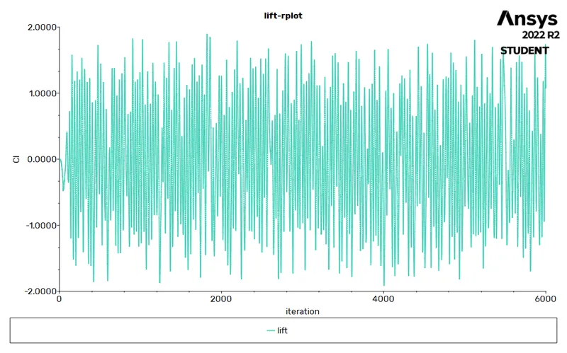
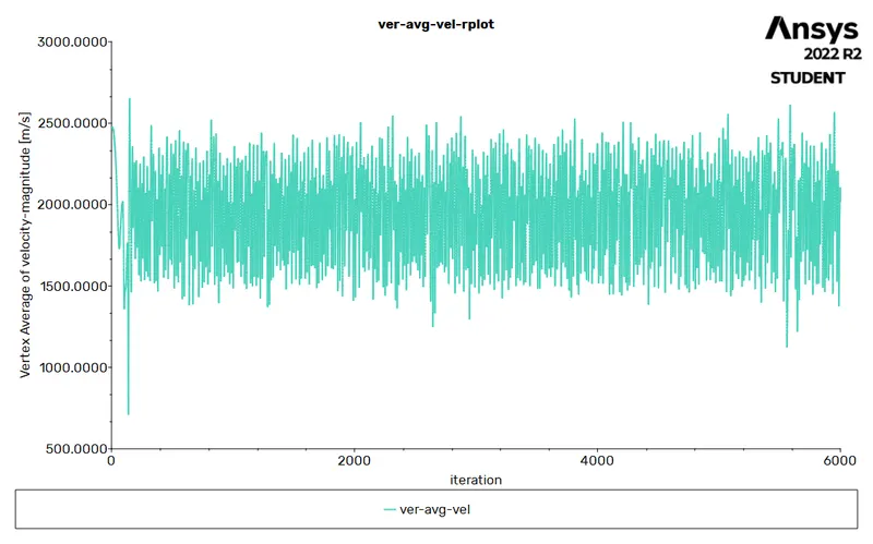
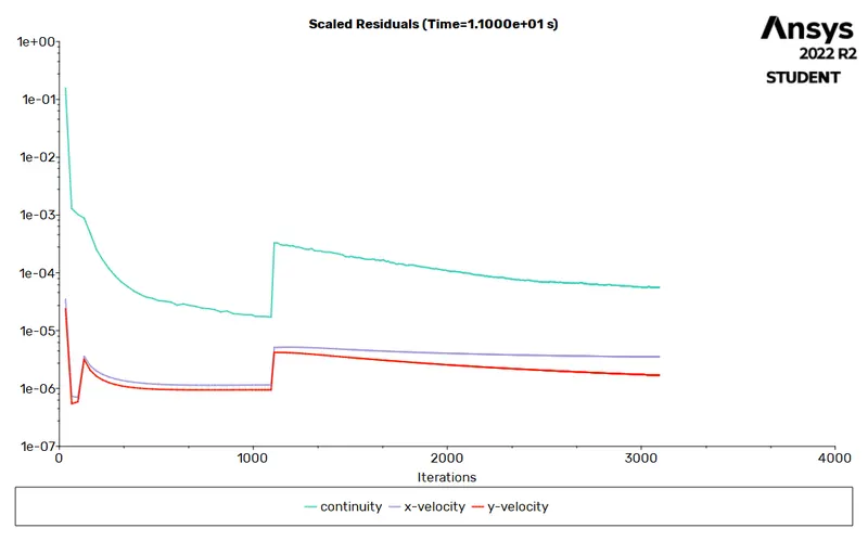
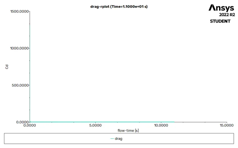
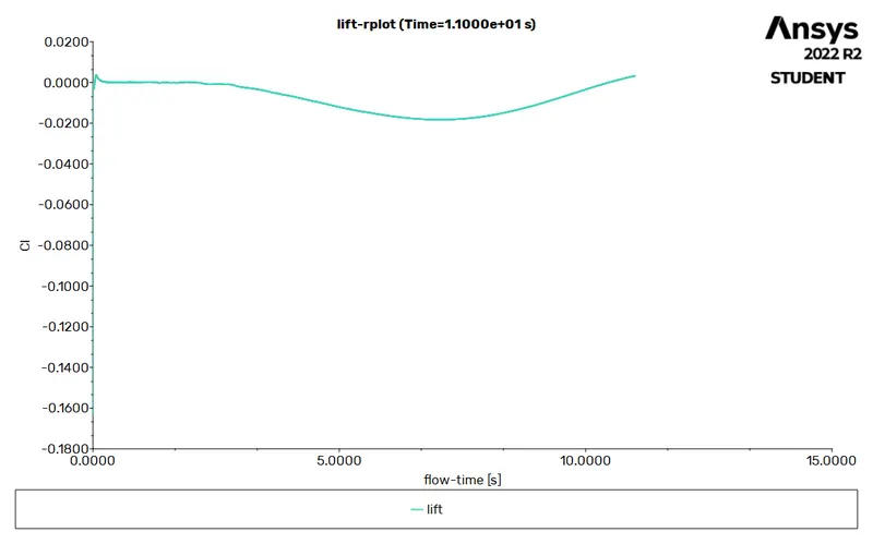
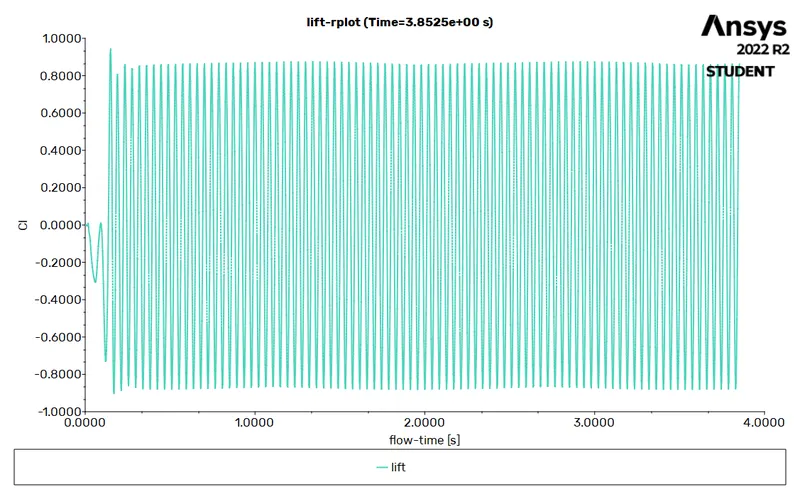
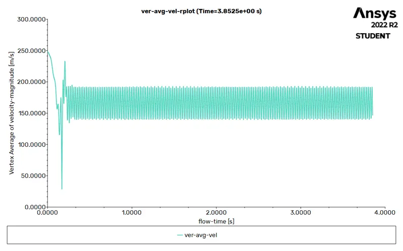
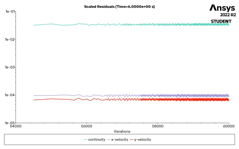
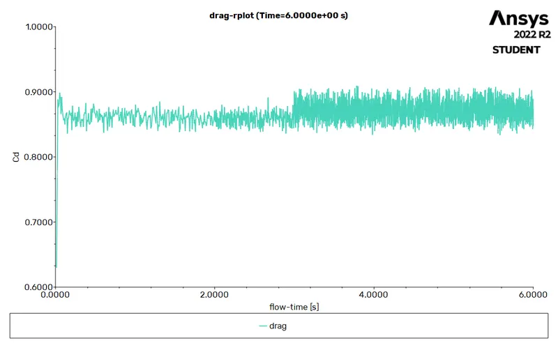
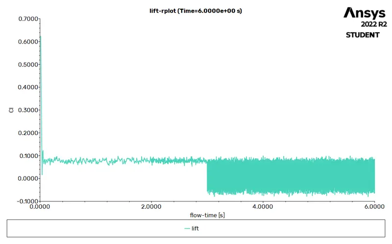
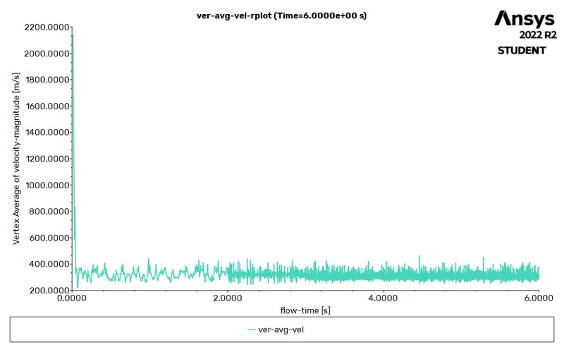
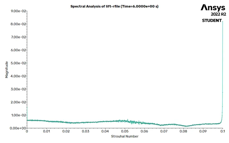
According to the problem statement, the Strouhal Number must be calculated for cases 6, 7, and 8, that is, for cases with transient state solver.

Results Toolbar > Plots > FFT > Y Axis Function - Magnitude & X Axis Function - Strouhal Number > Load Input File - 'Lift File' > Plot FFT > enable the 'Write FFT to File' > Write FFT

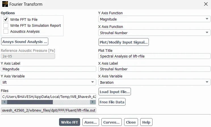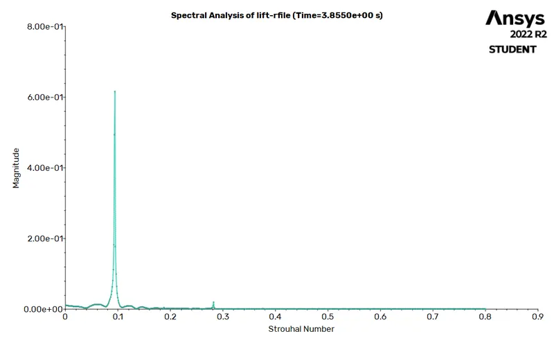
Thus, a plot and a file for the Strouhal number were produced. From the file, we extracted the value with maximum frequency as the Strauhol number.

Case No.	Strouhal Number Plot
6
7
8

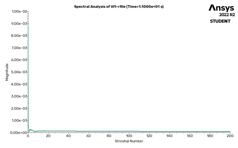
POST-PROCESSING -

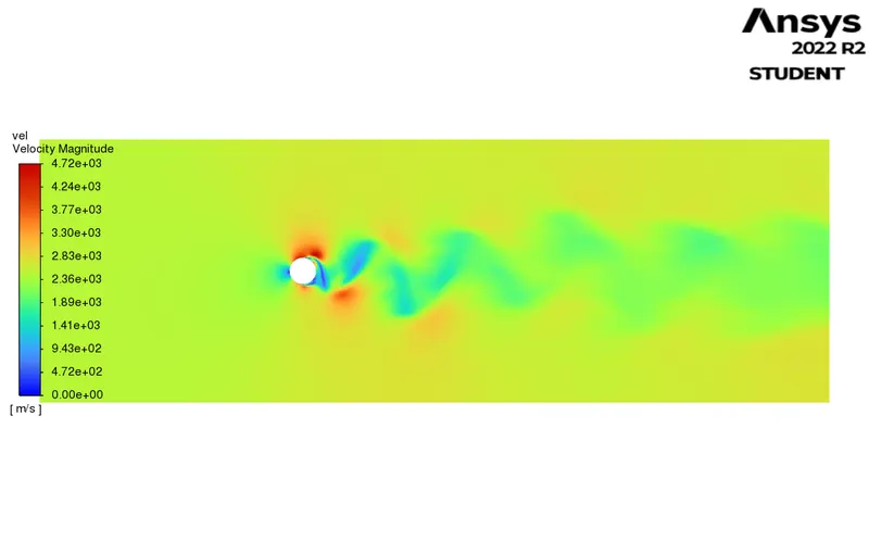
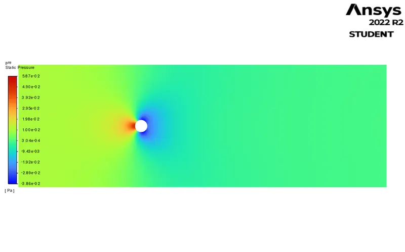
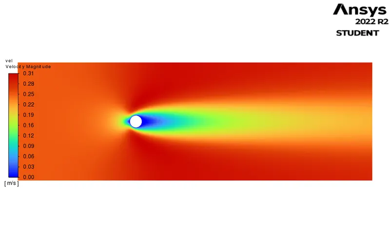
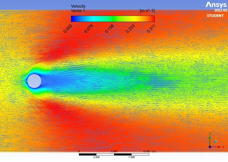
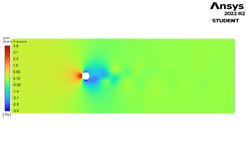
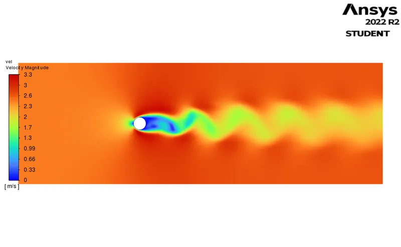
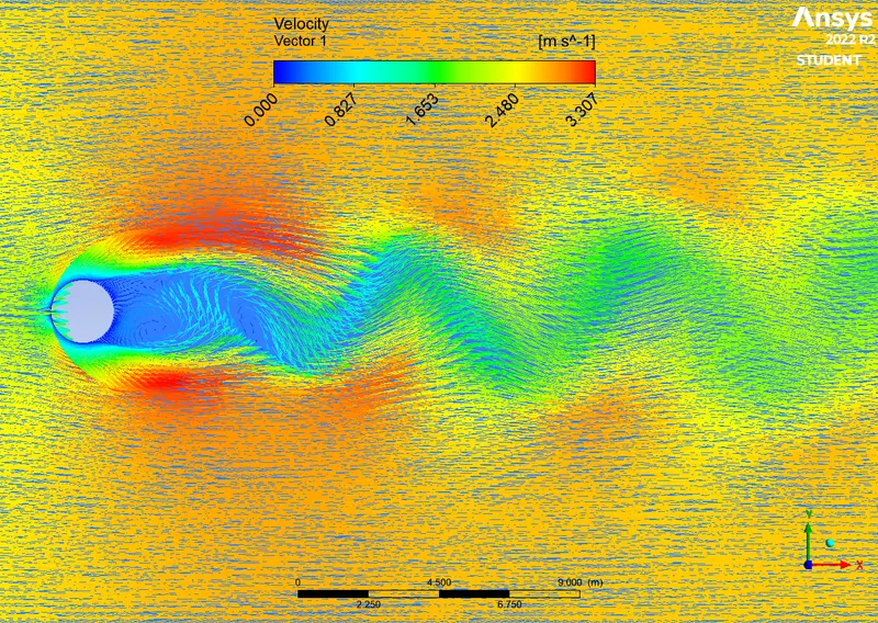
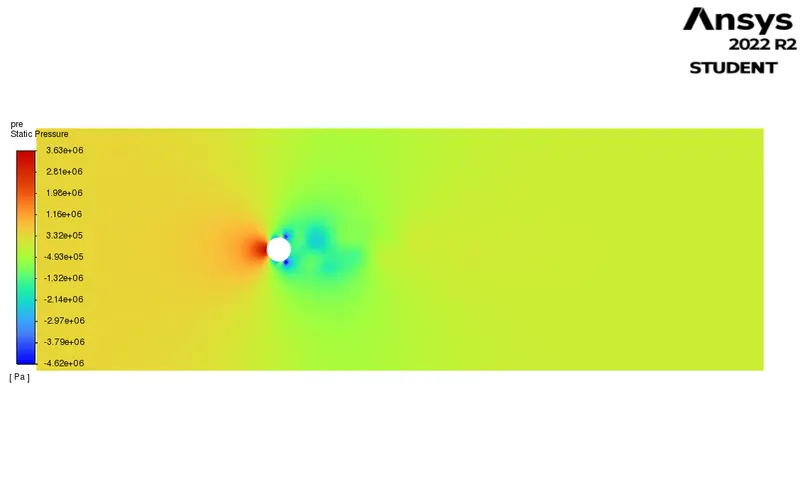
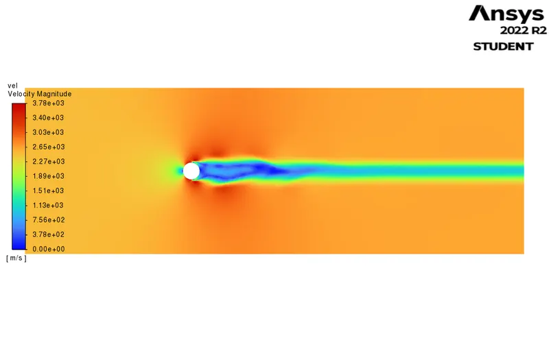
In post-processing, contours for pressure, velocity, and velocity vector over a plane parallel to the fluid flow were plotted.

RESULTS -

Case No.	Contours
	Pressure	Velocity	Velocity Vector (to observe the vortex shedding)
1
2
3
4
5
6
7
8

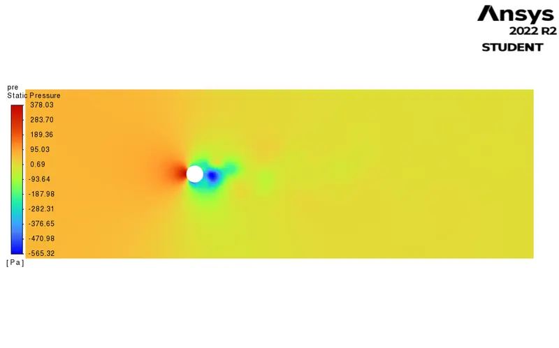
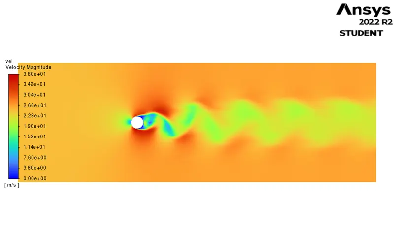
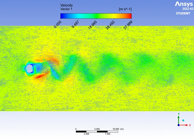
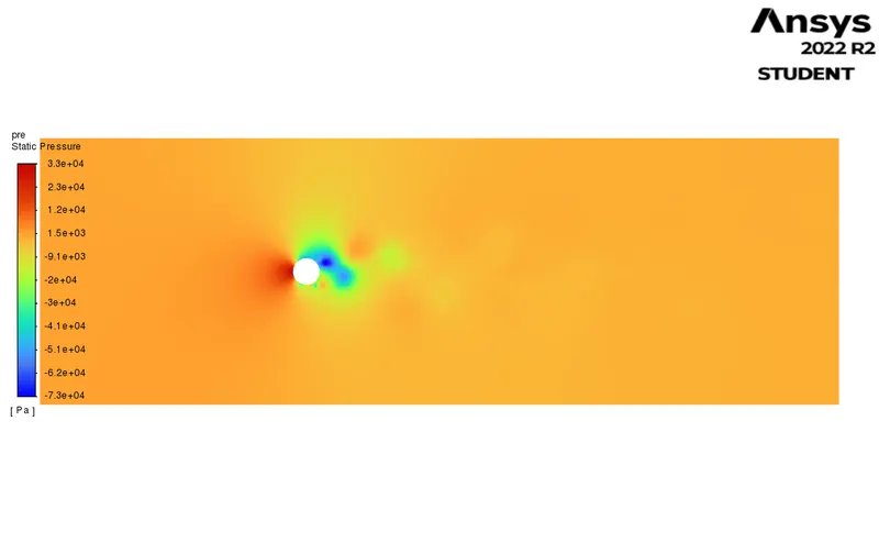
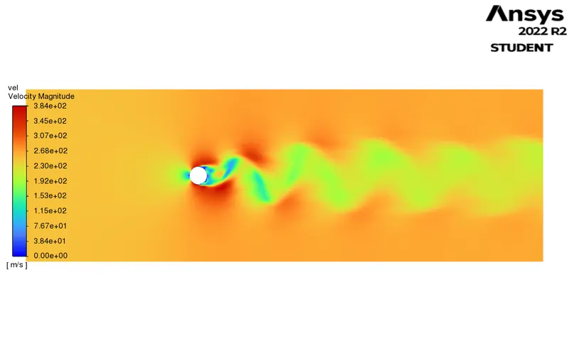
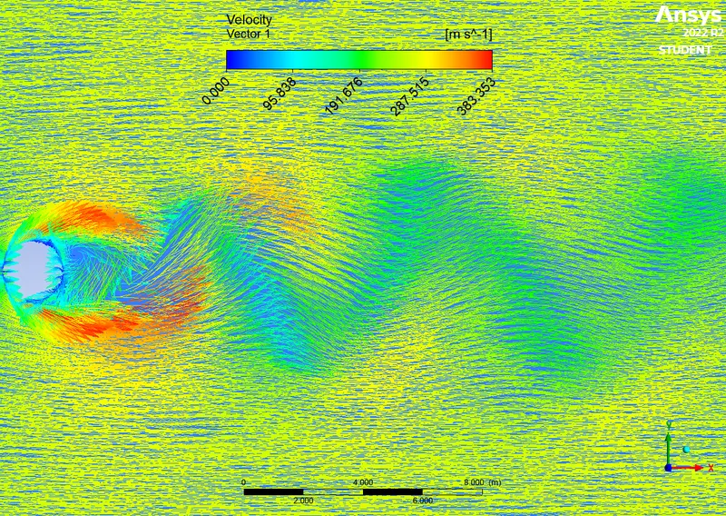
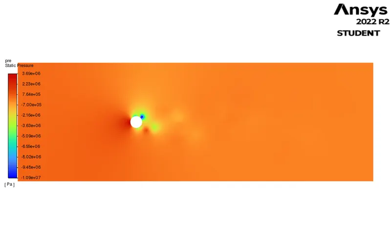
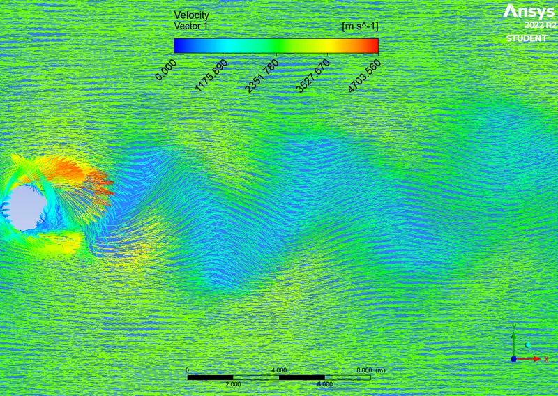
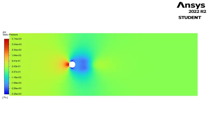
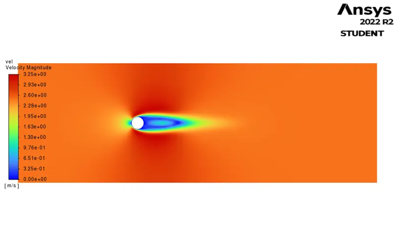
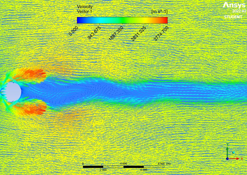
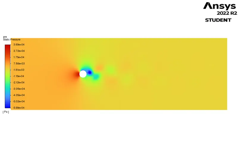
VALIDATION -

To validate our calculations, we used a graph from one of the reference books depicting the relationship between the Reynolds number (`Re`) and the Drag Coefficient (`C_D`) as;

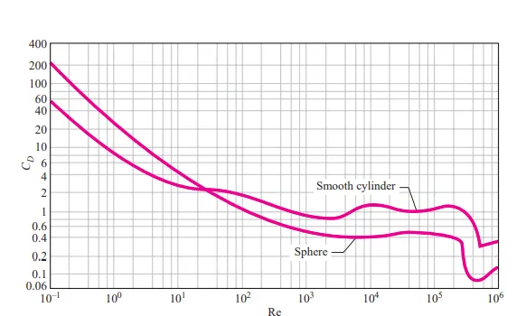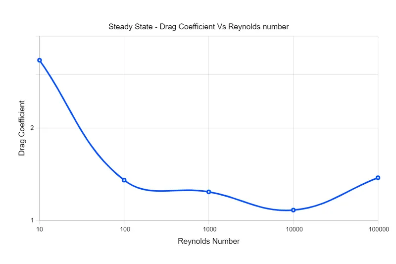
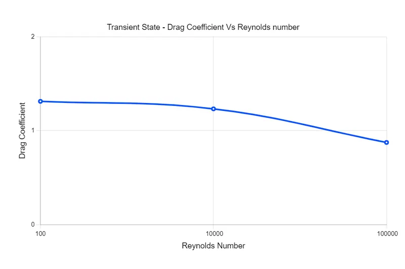
Based on the results, graphs between Reynolds Number and Drag Coefficient were plotted for both the steady state and transient state simulations, and when compared to the standard graph plot, the graphs were found to be relevant. As a result, it is possible to conclude that the simulation results were satisfactory.

Note: Because the cylinder's surface is very smooth and the geometry is symmetric, the lift will be minimal, and we haven't considered the lift coefficient in the validation.

CONCLUSION -

Outcomes for the simulation with Steady-state solver were;

Re	Drag Coefficient	Lift Coefficient	Vertex Average Velocity (m/s)
10	3.3366	-5.44e-05	0.1055
100	1.3542	-0.1370	0.9436
1000	1.2399	-0.4377	17.150
10000	1.0814	0.7191	221.94
100000	1.3789	1.0781	2017.0

Outcomes for the simulation with Transient-state solver were;

Re	Drag Coefficient	Lift Coefficient	Vertex Average Velocity (m/s)	Strouhal Number
100	1.3126	0.0032	0.7705	4.81e-04
10000	1.2326	0.8340	138.42	6.16e-01
100000	0.8750	-0.0630	292.62	8.19e-02

• The results of the simulation appeared to be relevant based on the relationship between the Drag Coefficient and the Reynolds number.
• We can see a decreasing trend in the drag coefficient value as the flow changes from laminar to turbulent, due to delayed flow separation.
• Contact between the object and the fluid decreases as the Reynolds number increases. As a result, the drag coefficient is decreased, which leads to an increase in the object's efficiency.
• Thus, it can be concluded that a variety of factors, such as the Reynolds number, the geometry of the object, the point of separation, etc., affect the values of the drag and lift coefficients.

REFERENCES -

• Fluid Mechanics - Fundamentals and Applications by Yunus A. Cengel & John M. Cimbala

Thus, for eight cases, simulations for external flow analysis over a cylinder were run, and conclusions were drawn based on the results.