Week 2 - Flow over a Cylinder.

Aim:

To Simulate the flow over a cylinder and explain the phenomenon of Karman vortex street.

Objective:

PART-I

1. Simulate the flow with the steady and unsteady case and calculate the Strouhal Number for Re= 100.

PART-II

1. Calculate the coefficient of drag and lift over a cylinder by setting the Reynolds number to 10,100,1000,10000 & 100000. (Run with steady solver)
2. Discuss the effect of the Reynolds number on the coefficient of drag.

Theory:

Karman vortex street

In fluid dynamics, a Kármán vortex street (or a von Kármán vortex street) is a repeating pattern of swirling vortices shedding, caused by a process known as vortex shedding, which is responsible for the unsteady separation of the flow of a fluid around blunt bodies. It is named after the engineer and fluid dynamicist Theodore von Karman.

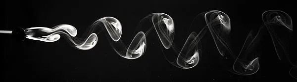
Vortex streets occur in liquids as well as gases. As fluids move toward a cylinder that is sticking up into the prevailing flow, that flow will split around the cylinder. The edge of the fluid that is in contact with the cylinder wall is slowed by friction. This will cause a spin in the flow on either side of the cylinder, creating eddies. Those eddies form in a regular pattern, first one, then the other on the downwind side of the object, and may continue to spin as they move downstream with the prevailing flow. The animation below shows the development of the vortices downwind of either side of the object.

Solving & Modelling Approach:

Geometry: -

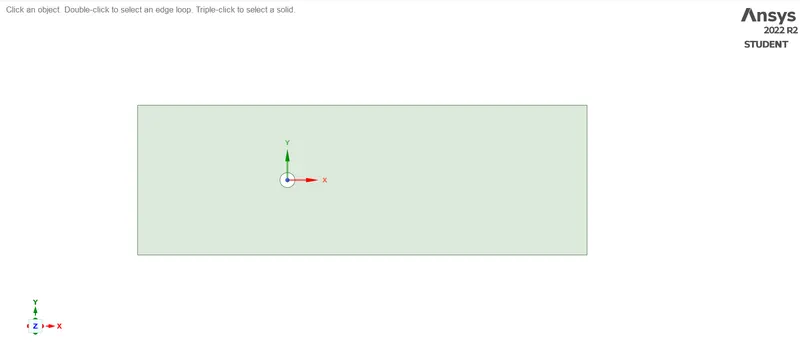
A plate with the dimension of 20*60m is created using SpaceClaim. we want to simulate the effect of fluid flow over the cylinder. The final geometry is shown below. To design the right physics the inside circular surface is to be deleted to carry out the simulation. Converting the geometry into the surface by using the command pull and select.

Meshing: -

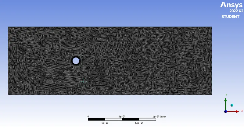
The meshing involves the creation of a small discrete domain for the calculation of governing equations. The mesh should be fine enough to compensate for every change that will create during the simulation. The Mesh size which is used for the steady state and unsteady solver will be the same which is 250mm for the overall domain. It is important to capture flow around the cylinder as flow separation seizure. To capture the flow near the cylinder the inflation layer is need to be used. Inflation will create a hexahedral mesh near the cylinder which makes solution convergence and will provide an accurate solution.

Before inflation layer creation is required to capture the boundary of the cylinder by using edge sizing. For edge sizing number of layers used is 36. The inflation layer property is the first layer thickness in which the height of the first layer is 5 mm and the number of layers is 20 for capturing more area near the cylinder with the growth rate of 1.2. After applying this value to the geometry the mesh will look like this:

Solution Setup:

Case 1: Steady flow simulation for Re = 10

Solver Type	Pressure Based
Velocity Formulation	Absolute
Time	Steady
Viscous Model	LAMINAR
Material	Fluid type: User-defined (Air) Where, viscosity = 0.05(kg m s) density = 1(kg/m^3)
Cell zones ff_surface	Fluid type: User-defined (Air)
Boundaries	Inlet (velocity inlet): Velocity Magnitude - 0.25 m/s Temperature – standard Outlet x (Pressure outlet): Gauge Pressure – 0 pascal Wall - wall: Symmetry - symmetry

Results:

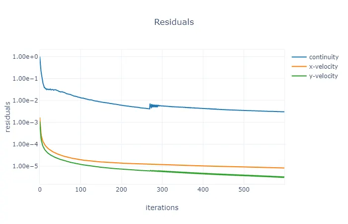
• Residual Plot:

• Vertex Average of Velocity Magnitude Plot:

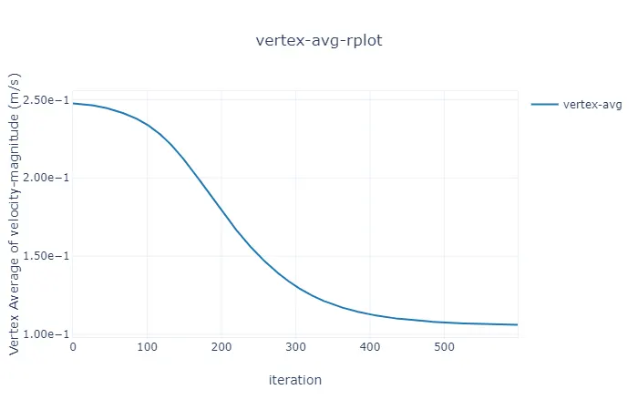
As the flow has very low velocity there are no fluctuations seen in the flow velocity at the designed vertex.

Vertex average velocity = 0.10610697 m/s

• Coefficient of Drag Plot:

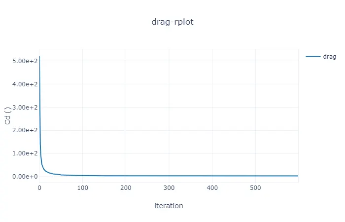
Due to the low-velocity drag coefficient, it shows a steady graph.

Drag Coefficient = 3.34

• Coefficient of Lift Plot:

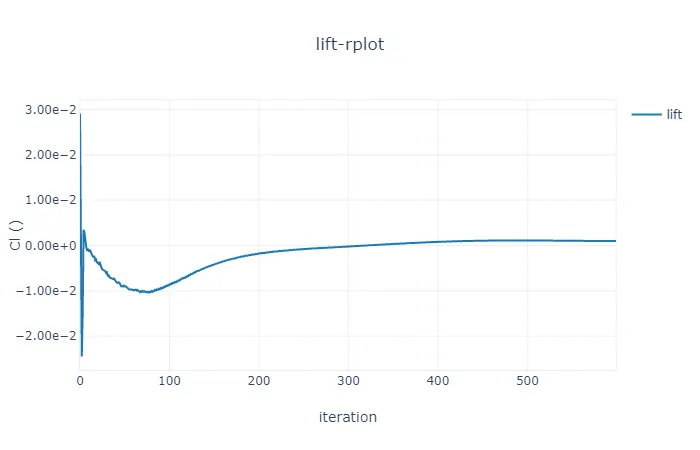
Due to the low-velocity lift coefficient is showing a steady graph.

Lift Coefficient = 0.00097

• Velocity Contour Plot:

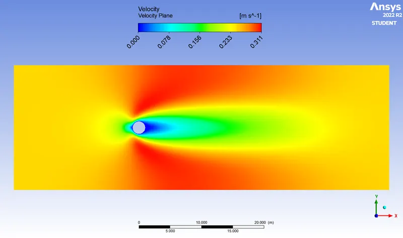
For Re = 10 no vortex shedding effect can be seen in the above velocity contours.

• Pressure Contour Plot:

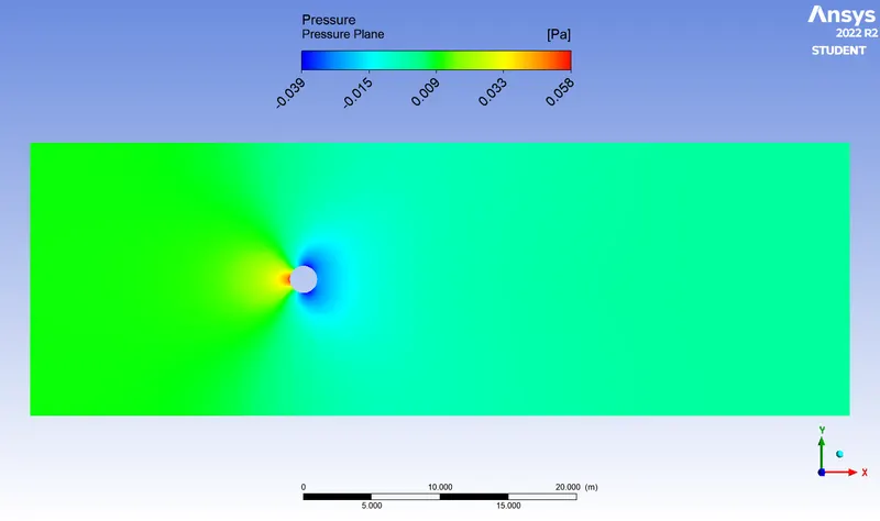
Pressure contours show the zone of impact which is a high-pressure zone within the region and it shows after flow impacts the cylinder the flow pressure reduces.

Case 2: Steady flow simulation for Re = 100

Solver Type	Pressure Based
Velocity Formulation	Absolute
Time	Steady
Viscous Model	LAMINAR
Material	Fluid type: User-defined (Air) Where, viscosity = 0.05(kg m s) density = 1(kg/m^3)
Cell zones ff_surface	Fluid type: User-defined (Air)
Boundaries	Inlet (velocity inlet): Velocity Magnitude - 2.5 m/s Temperature – standard Outlet x (Pressure outlet): Gauge Pressure – 0 pascal Wall - wall: Symmetry - symmetry

Results:

• Residual Plot:

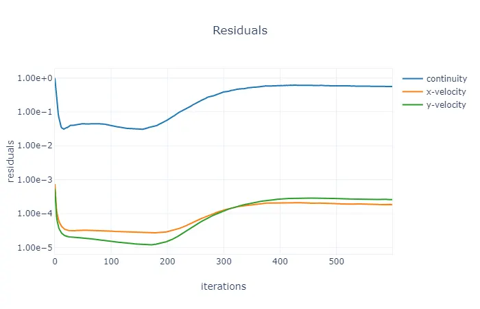
The above results show that the flow has reached a steady state as all the residuals are in steady and in straight lines.

• Vertex Average of Velocity Magnitude Plot:

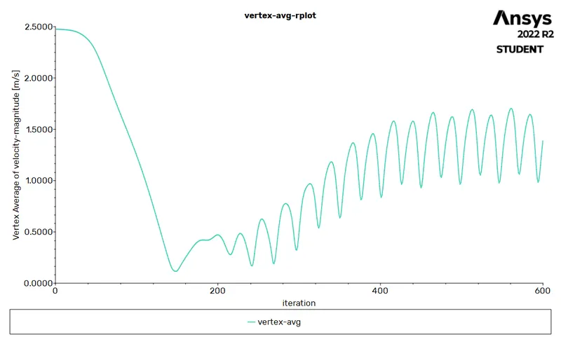
As the flow is showing the vortex shedding thus the velocity at the taken vertex keeps on fluctuating with the vortex flow which can be clearly seen in the graph.

Vertex average velocity = 1.3915043 m/s

• Coefficient of Drag Plot:

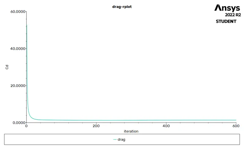
Due to the low-velocity drag coefficient, it shows a steady graph.

Drag Coefficient = 1.38

• Coefficient of Lift Plot:

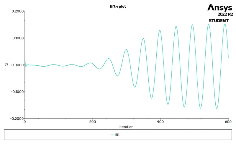
The lift coefficient shows a steadily fluctuating graph which is due to wake formation in a flow after cylinder.

Lift Coefficient = 0.026

• Velocity Contour Plot:

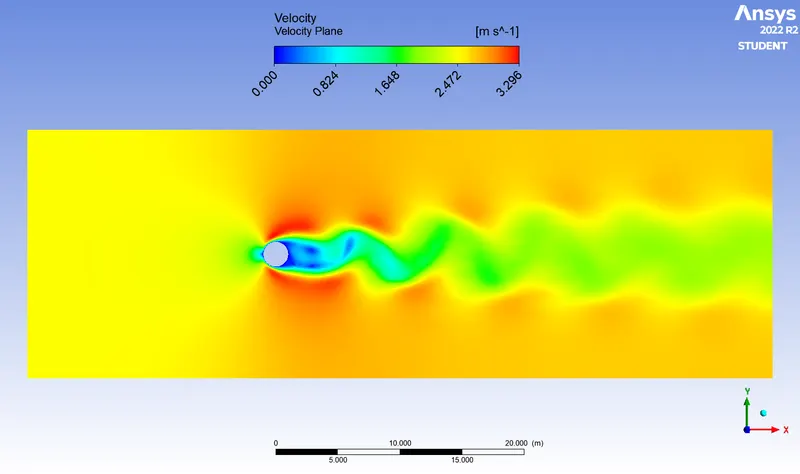
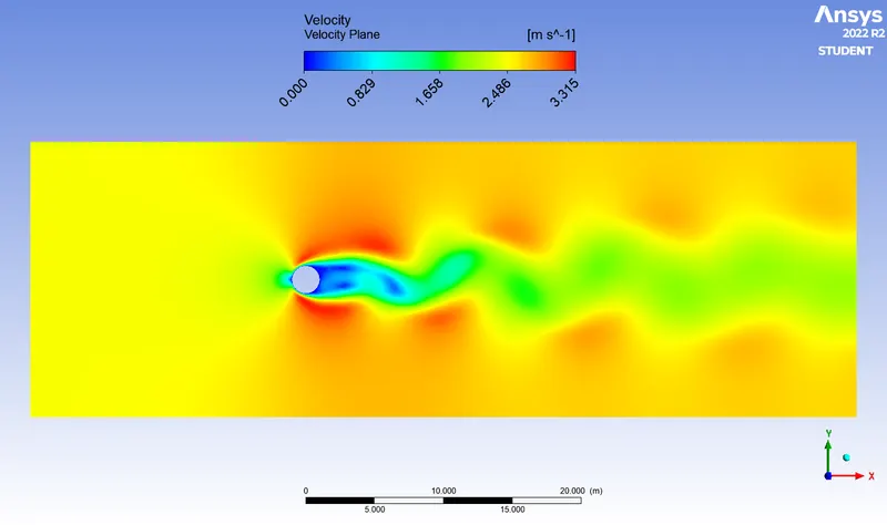
Velocity contours show that velocity distribution over a flow and there is a change in velocity within the region which is shown with the help of color contours. Thus the pattern of velocity shows vortex shedding behind the cylinder( shown by the green region). The vortex shedding size keeps on increasing with the distance traveled by the vortex.

• Pressure Contour Plot:

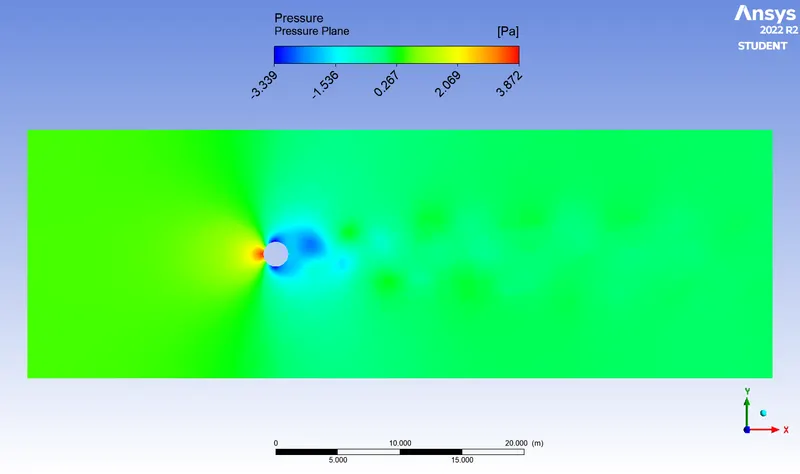
The above contours show the pressure distribution over an entire domain. Thus when flow impacts the cylinder high-pressure region is created and as we see around the cylinder due to flow separation the pressure is dropped behind and around the cylinder.

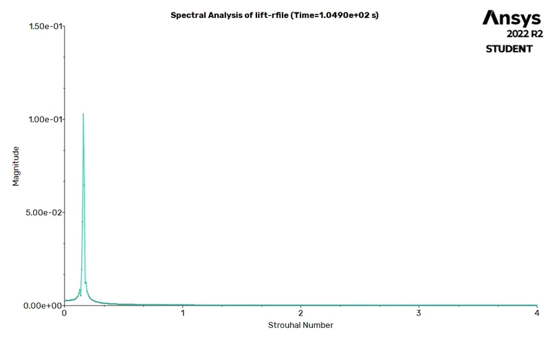
• Strouhal Number Plot:

The Strouhal Number is a dimensionless value useful for analyzing oscillating unsteady fluid flow dynamics problems.

Strouhal number cannot be calculated for the steady state as there is no time parameter that is required in frequency calculation and can only be calculated for unsteady state conditions.

Conclusion of Steady flow simulation for Re = 100:

In case Re = 100 Steady state simulation, the residuals become steady but they didn't fall below 1e-4 thus we go for checking the quantity of interest which is drag coefficient, lift coefficient, and avg. vertex velocity and the above graphs show that all the quantities are in a steady state hence we can say the solution is converged.

Case 3: Unsteady flow simulation for Re = 100

Solver Type	Pressure Based
Velocity Formulation	Absolute
Time	Transient (Unsteady)
Viscous Model	LAMINAR
Material	Fluid type: User-defined (Air) Where, viscosity = 0.05(kg m s) density = 1(kg/m^3)
Cell zones ff_surface	Fluid type: User-defined (Air)
Boundaries	Inlet (velocity inlet): Velocity Magnitude - 2.5 m/s Temperature – standard Outlet x (Pressure outlet): Gauge Pressure – 0 pascal Wall - wall: Symmetry - symmetry

Results:

• Residual Plot:

• Vertex Average of Velocity Magnitude Plot:

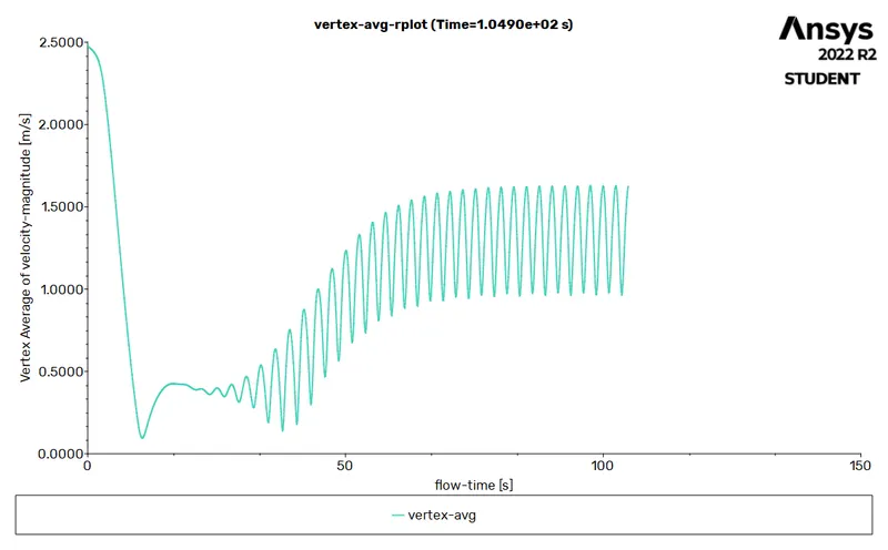
As the flow is showing the vortex shedding thus the velocity at the taken vertex keeps on fluctuating with the vortex flow which can be clearly seen in the graph.

Vertex average velocity = 1.6262633 m/s

• Coefficient of Drag Plot:

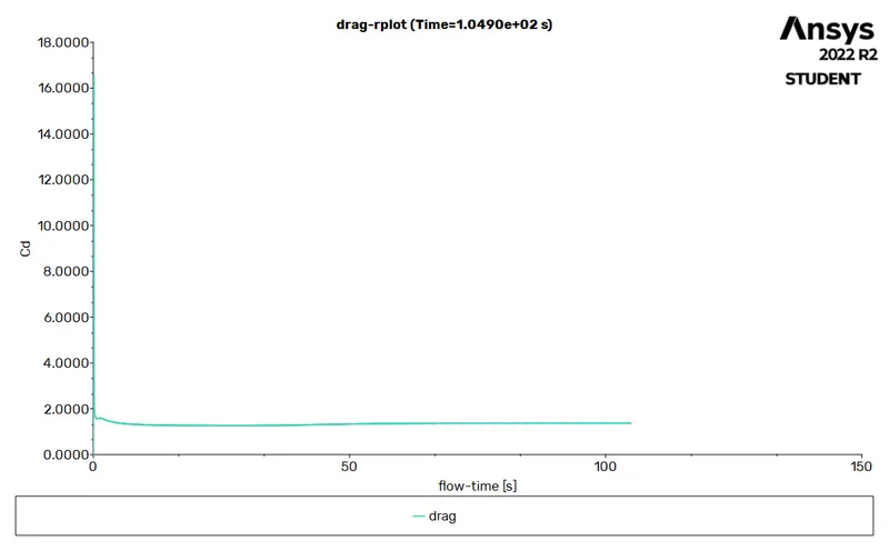
Due to the low-velocity drag coefficient, it shows a steady graph.

Drag Coefficient = 1.37

• Coefficient of Lift Plot:

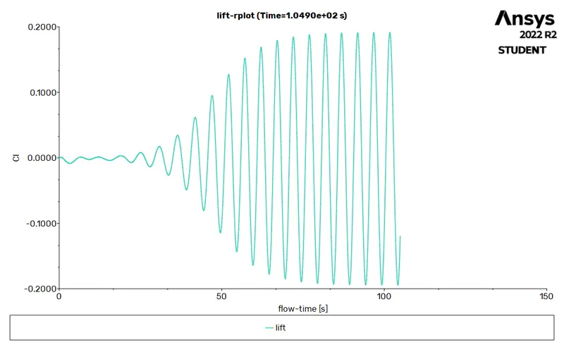
As in an unsteady state, simulation time is considered i.e. simulation is recorded from t= 0 to t= taken time thus the change for every time step is recorded therefore we can see in the lift coefficient graph that its fluctuation amplitude keeps on increasing till it becomes steady.

Lift Coefficient = 0.120008

• Velocity Contour Plot:

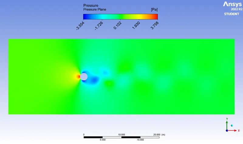
• Pressure Contour Plot:

• Strouhal Number Plot:

The Strouhal Number is a dimensionless value useful for analyzing oscillating unsteady fluid flow dynamics problems.

The Strouhal number is often given as

where St = Strouhal Number

f = oscillation frequency

L = characteristic frequency

U = flow velocity

Hence, the theoretical value of strouhal number is...

Since, f = No.of peaks/Flow time = 3/20 = 1.5Hz

Therefore, St = (1.5 * 2) / 1 = 0.3

Now, the theoretical value of the strouhal number is 0.1996

Conclusion of Steady flow simulation for Re = 100:

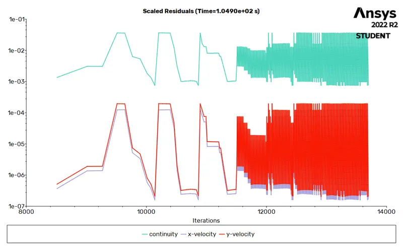
In case Re = 100 unsteady state simulation, the residuals are steadily fluctuating but again all of them didn't fall below 1e-4 thus after checking the quantity of interest we can say that solution is converged.

Case 4: Steady flow simulation for Re = 1000

Solver Type	Pressure Based
Velocity Formulation	Absolute
Time	Steady
Viscous Model	LAMINAR
Material	Fluid type: User-defined (Air) Where, viscosity = 0.05(kg m s) density = 1(kg/m^3)
Cell zones ff_surface	Fluid type: User-defined (Air)
Boundaries	Inlet (velocity inlet): Velocity Magnitude - 25 m/s Temperature – standard Outlet x (Pressure outlet): Gauge Pressure – 0 pascal Wall - wall: Symmetry - symmetry

Results:

• Residual Plot:

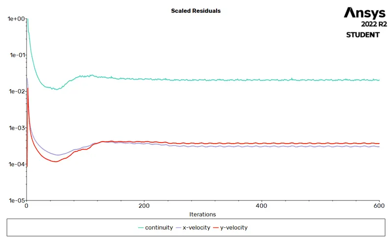
From the steady residuals graph, we can say that flow has converged.

• Vertex Average of Velocity Magnitude Plot:

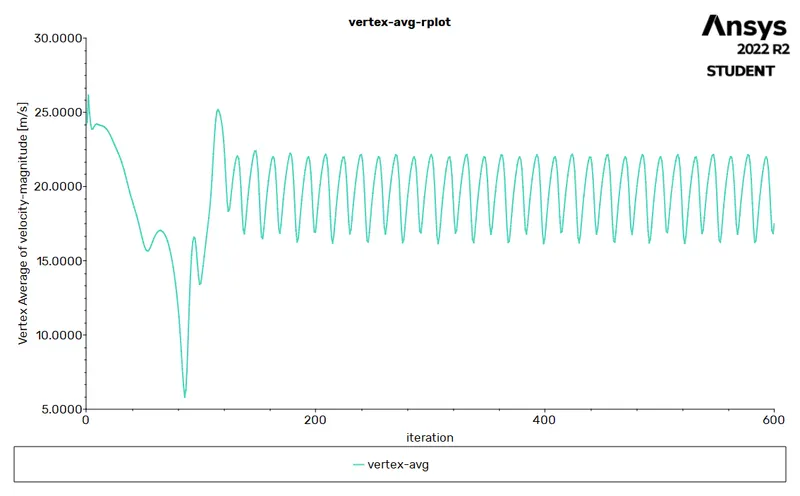
From steadily fluctuating avg. vertex velocity we can say that flow has converged.

Vertex average velocity = 17.491945 m/s

• Coefficient of Drag Plot:

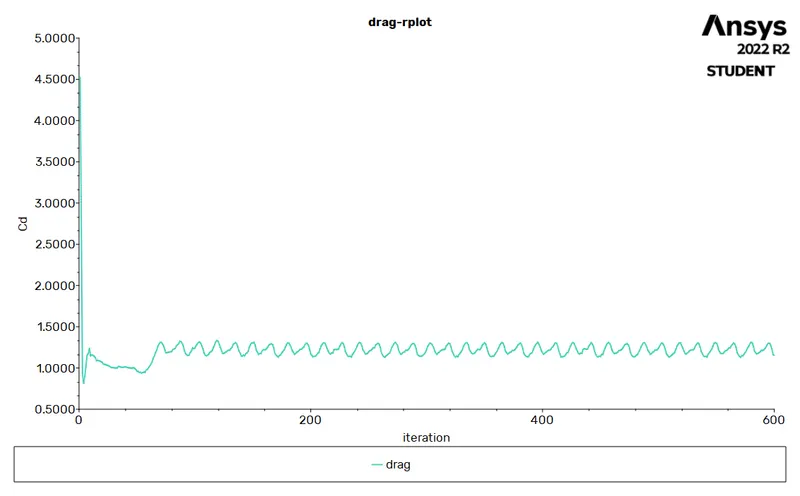
From the steadily fluctuating coefficient of the drag graph, we can say that flow has converged.

Drag Coefficient = 1.15

• Coefficient of Lift Plot:

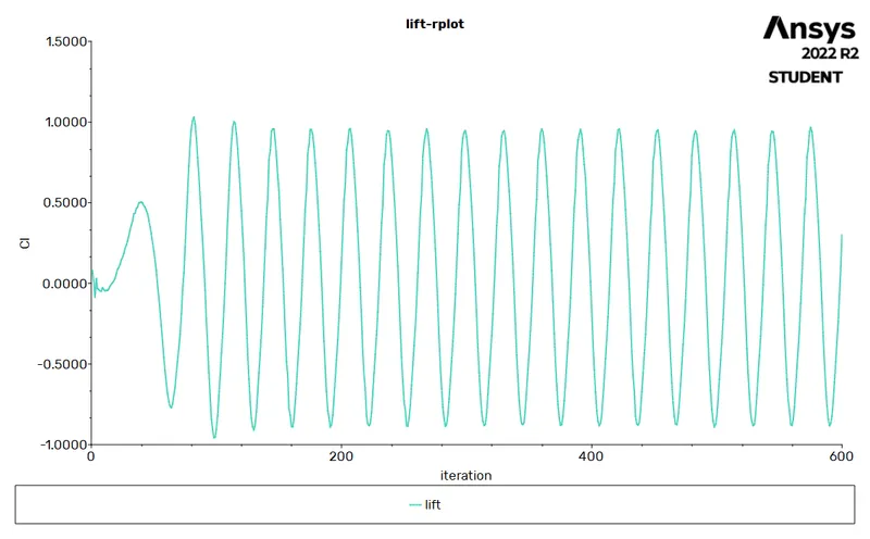
From the steadily fluctuating coefficient of lift graph, we can say that flow has converged.

Lift Coefficient = 0.29917711

• Velocity Contour Plot:

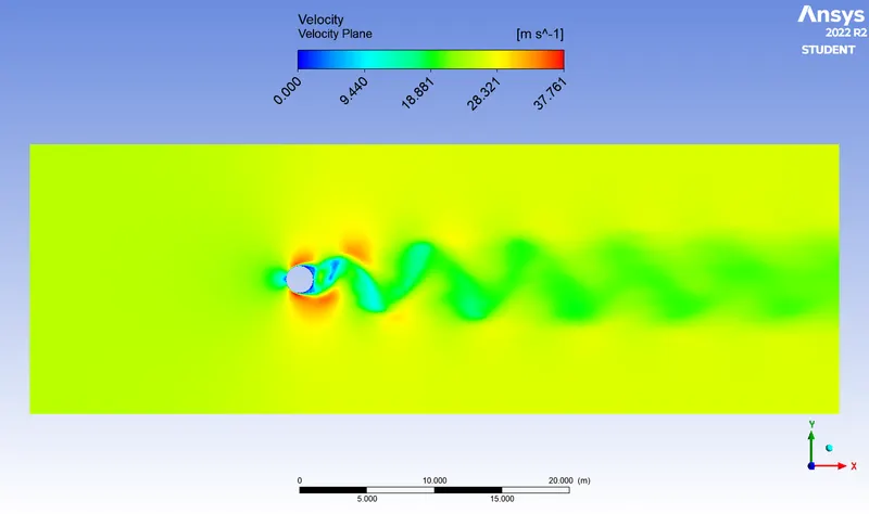
For Re = 1000 we can see in velocity contours that the faster vortex shedding takes place as the velocity of the flow increases but the vortex height is reduced as compared to Re = 100.

• Pressure Contour Plot:

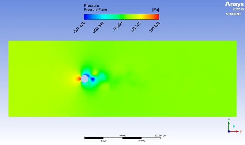
Pressure contours show that as the flow velocity increases static pressure zone increases with the and flow separation increases.

Case 5: Steady flow simulation for Re = 10000

Solver Type	Pressure Based
Velocity Formulation	Absolute
Time	Steady
Viscous Model	LAMINAR
Material	Fluid type: User-defined (Air) Where, viscosity = 0.05(kg m s) density = 1(kg/m^3)
Cell zones ff_surface	Fluid type: User-defined (Air)
Boundaries	Inlet (velocity inlet): Velocity Magnitude - 250 m/s Temperature – standard Outlet x (Pressure outlet): Gauge Pressure – 0 pascal Wall - wall: Symmetry - symmetry

Results:

• Residual Plot:

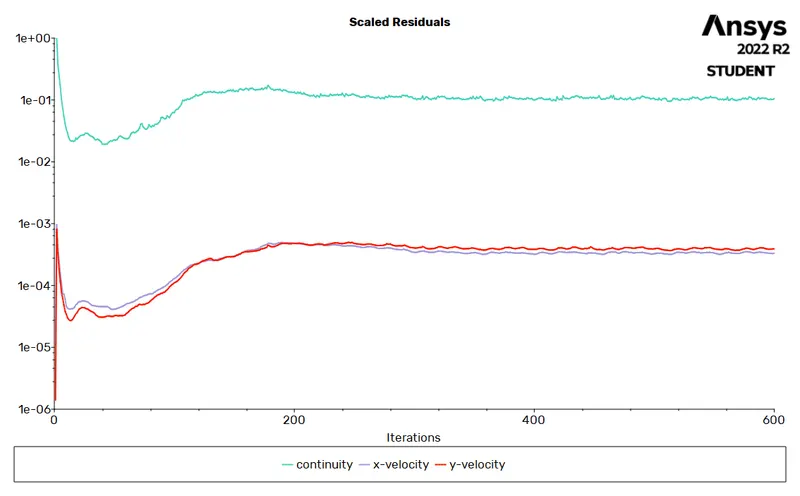
From steady residuals, we can say that flow has converged.

• Vertex Average of Velocity Magnitude Plot:

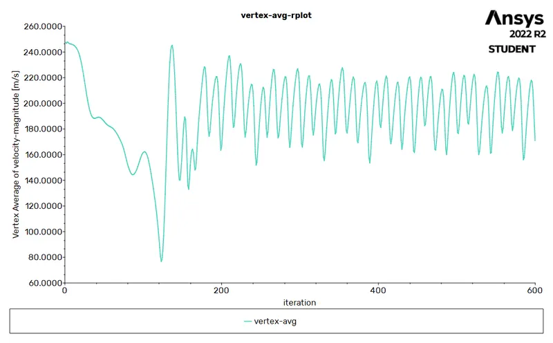
From steadily fluctuating avg. vertex velocity we can say that flow has converged. As the flow Reynolds no. increases the fluctuation in the vortex gets faster which can be clearly seen in the vertex avg. velocity graph.

Vertex average velocity = 170.79477 m/s

• Coefficient of Drag Plot:

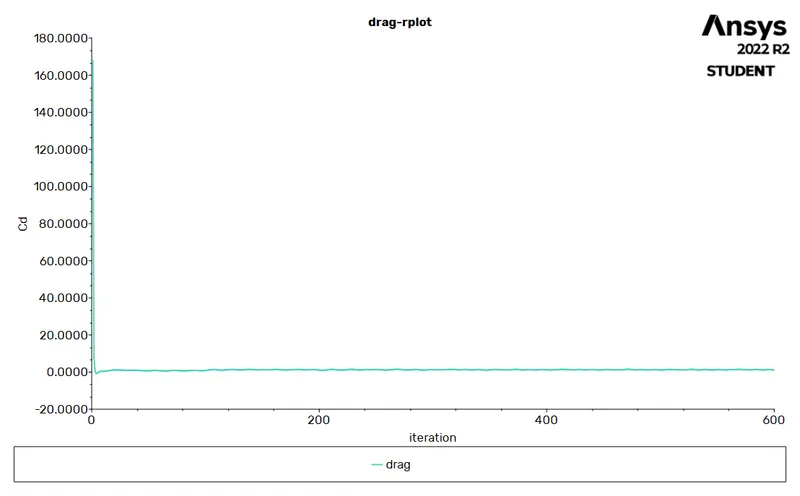
From the steadily fluctuating coefficient of the drag graph, we can say that flow has converged.

Drag Coefficient = 1.104

• Coefficient of Lift Plot:

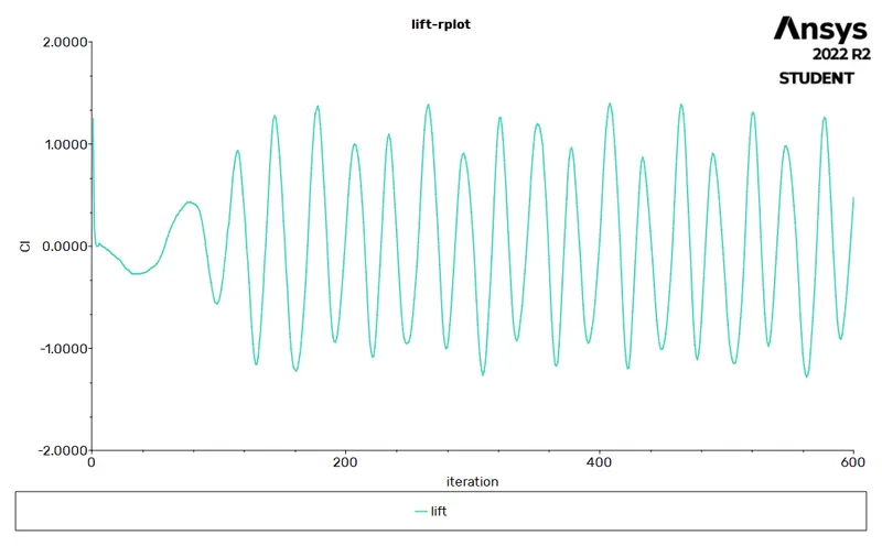
From the steadily fluctuating coefficient of lift, we can say that flow has converged. As the flow Reynolds no. increases the fluctuation in the vortex gets faster which can be clearly seen in the lift coefficient graph.

Lift Coefficient = 0.47540

• Velocity Contour Plot:

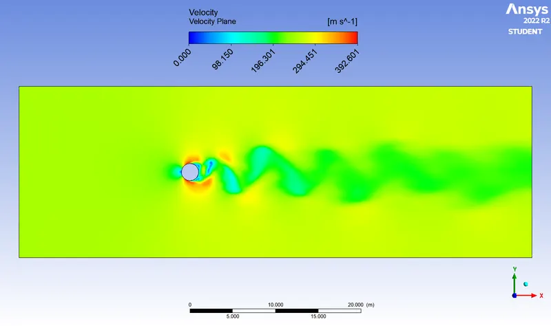
As the Reynolds no. increases to 10000 the vortex shedding effect gets more faster but the effect of vortex street size keeps on decreasing.

• Pressure Contour Plot:

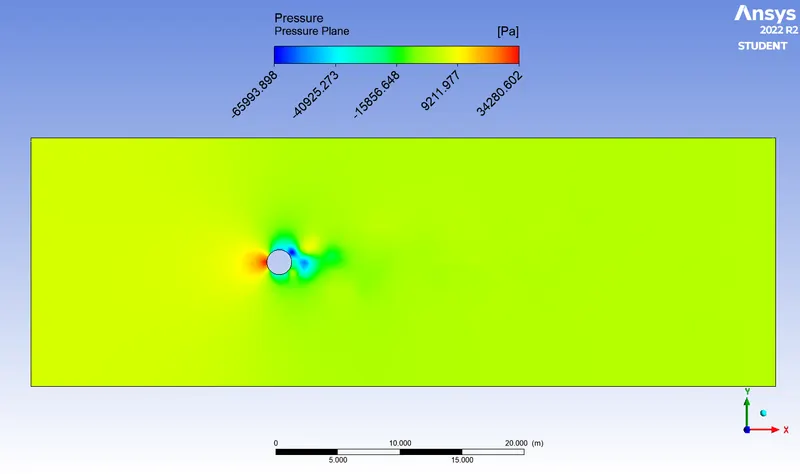
As the Reynolds no. increases to 10000 the pressure of impact decreases and flow separation increases.

Case 6: Steady flow simulation for Re = 100000

Solver Type	Pressure Based
Velocity Formulation	Absolute
Time	Steady
Viscous Model	LAMINAR
Material	Fluid type: User-defined (Air) Where, viscosity = 0.05(kg m s) density = 1(kg/m^3)
Cell zones ff_surface	Fluid type: User-defined (Air)
Boundaries	Inlet (velocity inlet): Velocity Magnitude - 2500 m/s Temperature – standard Outlet (Pressure outlet): Gauge Pressure – 0 pascal Wall - wall: Symmetry - symmetry

Results:

• Residual Plot:

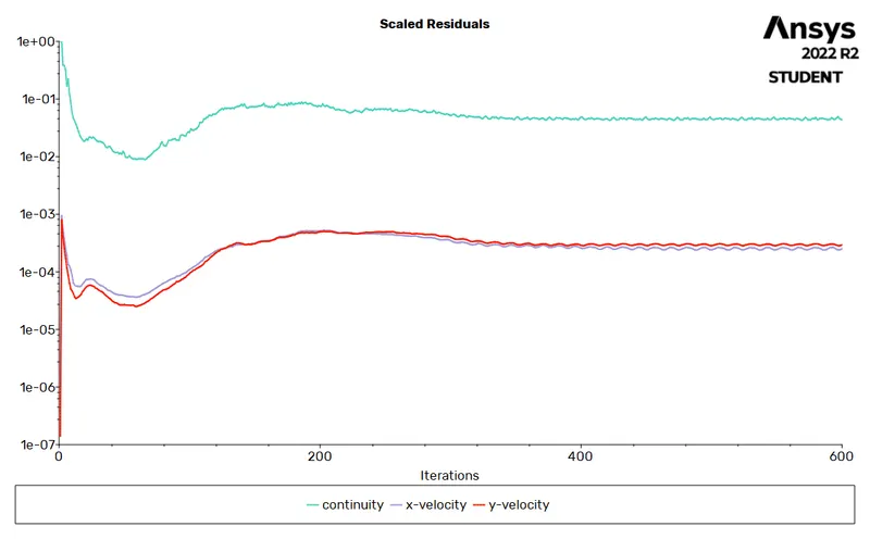
From steady residuals, we can say that flow has converged.

• Vertex Average of Velocity Magnitude Plot:

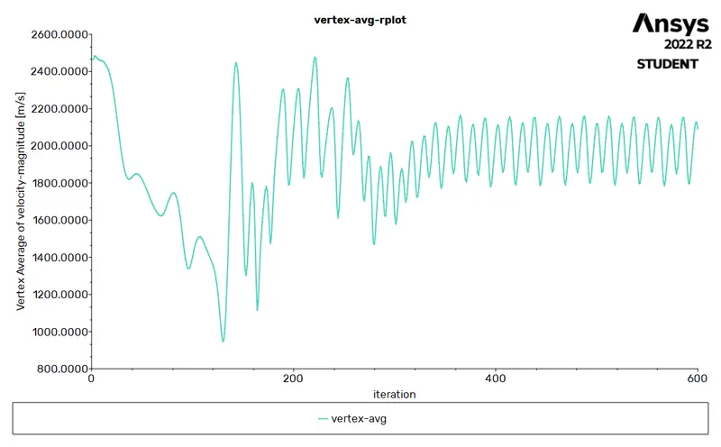
From steadily fluctuating avg. vertex velocity we can say that flow has converged. As the flow Reynolds no. increases the fluctuation in the vortex gets faster which can be clearly seen in the vertex avg. velocity graph.

Vertex average velocity = 2089.4316 m/s

• Coefficient of Drag Plot:

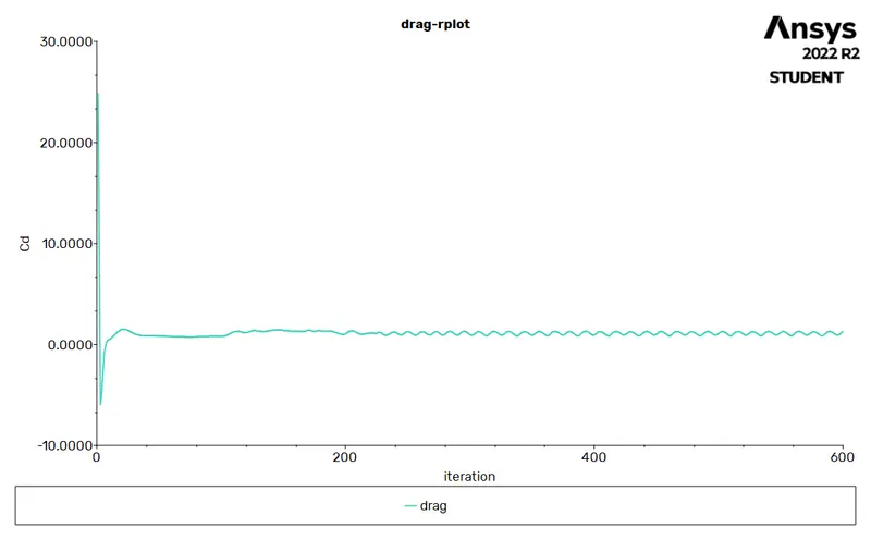
From the steadily fluctuating coefficient of the drag graph, we can say that flow has converged.

Drag Coefficient = 1.25

• Coefficient of Lift Plot:

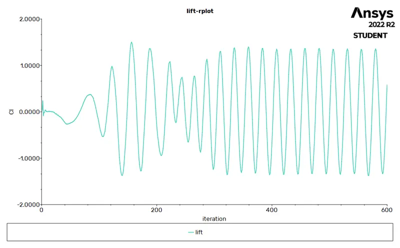
From the steadily fluctuating coefficient of lift, we can say that flow has converged. As the flow Reynolds no. increases the fluctuation in the vortex gets faster which can be clearly seen in the lift coefficient graph.

Lift Coefficient = 0.57940

• Velocity Contour Plot:

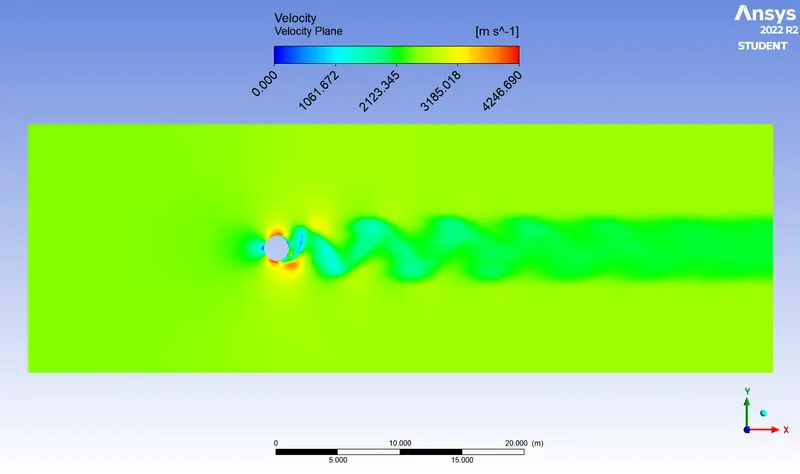
As the Reynolds no. increases to 10000 the vortex shedding effect gets more faster but the effect of vortex street size keeps on decreasing.

• Pressure Contour Plot:

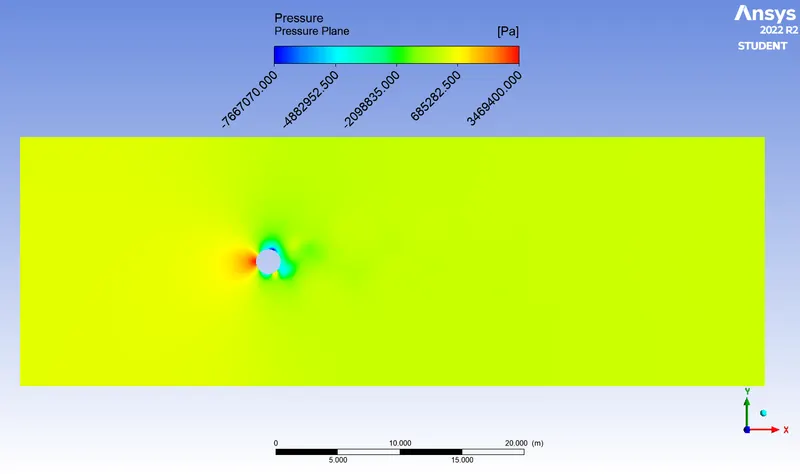
As the Reynolds no. increases to 10000 the pressure of impact decreases and flow separation increases.

Overall Result:

Reynolds Number	Drag Coefficient	Lift Coefficient	Average vertex velocity
10	3.34	0.00097	0.10610697
100 (Steady State)	1.38	0.02597	1.3915043
100 (Unsteady State)	1.37	0.120008	1.6262633
1000	1.15	0.29917	17.491945
10000	1.104	0.47540	170.79477
100000	1.25	0.57940	2089.4316

Overall Conclusions:

1. Comparing the steady state and unsteady state solvers for the same Reynolds no. Steady-state records the activities as the flow gets stable there is no time factor consideration taking place where as for unsteady-state the activities of flow are recorded starting from t = 0. Thus these activities are accordingly captured in the given graphs and contours.
2. For RE = 10 no vortex-shedding street is seen. As we increase the Reynolds no. from 100 to 1000 the vortex shedding street is effectively seen. and for Re = 10000 the vortex shedding is very less and street formation is not prominent but for Re = 100000 the vortex street with a very small height can be seen.
3. As the Reynolds no. increases the coefficient of drag decreases and the Lift coefficient increases but for Re = 10000 things get slightly changed the drag slightly increases and for Re = 100000 lift is slightly decreased.