Week 2 - Flow over a Cylinder.

Simulate the flow over a cylinder and explain the phenomenon of Karman vortex street

Aim:To simulate the flow over a cylinder and explain the phenomenon of Karman vortex street.

Objectives:

1. To simulate the flow with the steady and unsteady case and calculate the Strouhal Number for Re= 100. (Part-I)
2. To calculate the coefficient of drag and lift over a cylinder by setting the Reynolds number to 10,100,1000,10000 & 100000. (Run with steady solver) (Part-II)
3. To discuss the effect of Reynolds number on the coefficient of drag.

Introduction:This study is to analyze the flow over a cylinder with laminar flow (assumed), but our main interest is to look for the formation of von karman vortex street in steady and unsteady flow nature using ansys-fluent.

Theory: The real flow over a cylinder is unlike an ideal inviscid flow over the cylinder having net zero drag by d’alembert’s paradox. It will have a boundary layer adjacent to surface of the bluff body of study and also the boundary layer separation occurs which will tend to form a wake region downstream of the flow which will be a low pressure region resulting in drag on that body in downstream direction.

The resultant flow is an oscillated flow by having an periodical formation of low pressure regions of same pattern in an oscillated manner in the downstream. The low pressure regions are in the form fluid circulating region where at the center of the region there will be a void space due to this flow circulation happens but this region disappears on spatial marching in downstream flow direction.

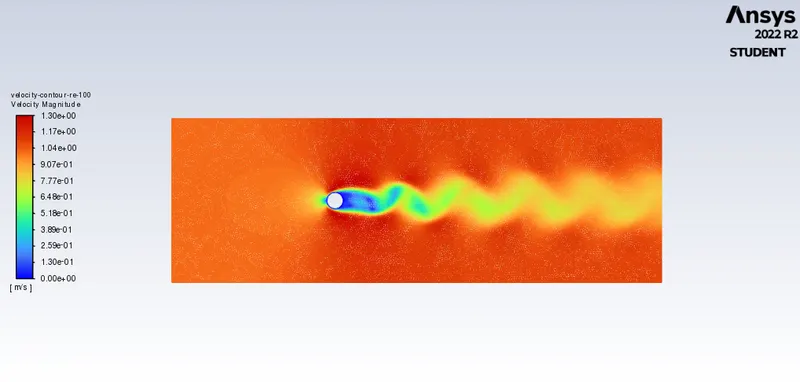
This is called as vortices and this vortices follows a regular pattern based on the flow velocity, shape and size of the body. This pattern of formation of vortices repeatedly in an oscillating manner is called as vortex shedding and the downstream region of bluff body is called as Vortex Street.

In fluid dynamics, a Kármán vortex street (or a von Kármán vortex street) is a repeating pattern of swirling vortices shedding, caused by a process known as vortex shedding, which is responsible for the unsteady seperation of flow of a fluid around blunt bodies. It is named after the engineer and fluid dynamicist Theodore von Karman.

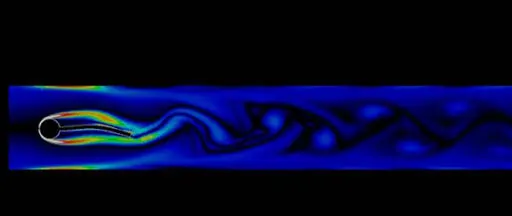
As a fluid particle flows toward the leading edge of a cylinder, the pressure on the particle rises from the free stream pressure to the stagnation pressure. The high fluid pressure near the leading edge impels flow about the cylinder as boundary layers develop about both sides. The high pressure is not sufficient to force the flow about the back of the cylinder at high Reynolds numbers. Near the widest section of the cylinder, the boundary layers separate from each side of the cylinder surface and form two shear layers that trail aft in the flow and bound the wake. Since the innermost portion of the shear layers, which is in contact with the cylinder, moves much more slowly than the outermost portion of the shear layers, which is in contact with the free flow, the shear layers roll into the near wake, where they fold on each other and coalesce into discrete swirling vortices. A regular pattern of vortices called a vortex street trails aft in the wake.

The frequency of the oscillated flow ( vortex shedding ) is used to determine the effect of the vortices formed, that frequency is related to the strouhal number which is a dimensionless number.

St = f*D/V

St – strouhal number of the vortex shedding.

f – Frequency of vortex shedding

D – Characteristic length of the bluff body

V – Free stream velocity

Modelling and solving approach:

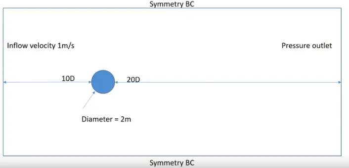
1.Creating Geometry:(unit is set to meters using spaceclaim option)

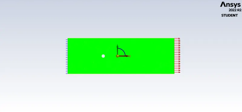
• Creating the geometry by sketching using the line and circle command, circle diameter of 2m and the dimensions having 20X60m and the circle is placed 20m from the inlet.

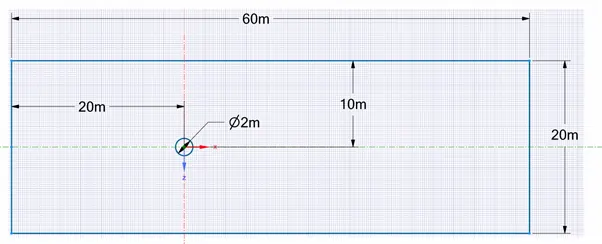
• There is no thickness provided to the geometry as it is a 2D simulation. After providing the details the geometry will be:

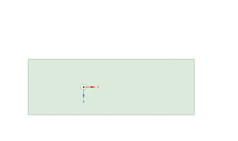
2.Creating Mesh:

• Mesh should be fine enough to compensate for every changes that will create during simulation. Mesh size which is used for the steady state and unsteady solver will be same which is 0.25m for overall domain. It is important to capture flow around cylinder as flow separation seizure.
• To capture the flow near cylinder the inflation layer is need to be used. Inflation will create hexahedral mesh near the cylinder which makes solution convergence and will provide accurate solution.

Before inflation layer creation it required to capture the boundary of cylinder by using edge sizing local meshing method. For edge sizing no. of divisions can be used as user input. For this case division is taken as 36. The inflation layer property is first layer thickness in which height of first layer is 0.005 m and amount of layer are 6 for capturing more area near the cylinder with growth rate of 1.2.

Boundaries are set using named selection:

inlet,outlet,wall,symmetry boundary.

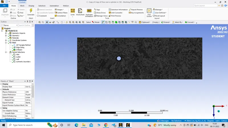
3.Making set up:

• Steady case for Re= 100. (Part-I)

• Setting the solver:time:Steady
• Method:hybrid
• no of iteration=500

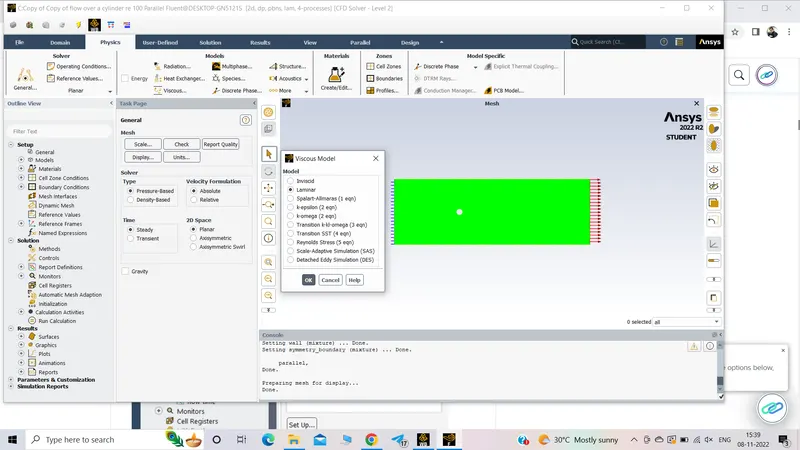
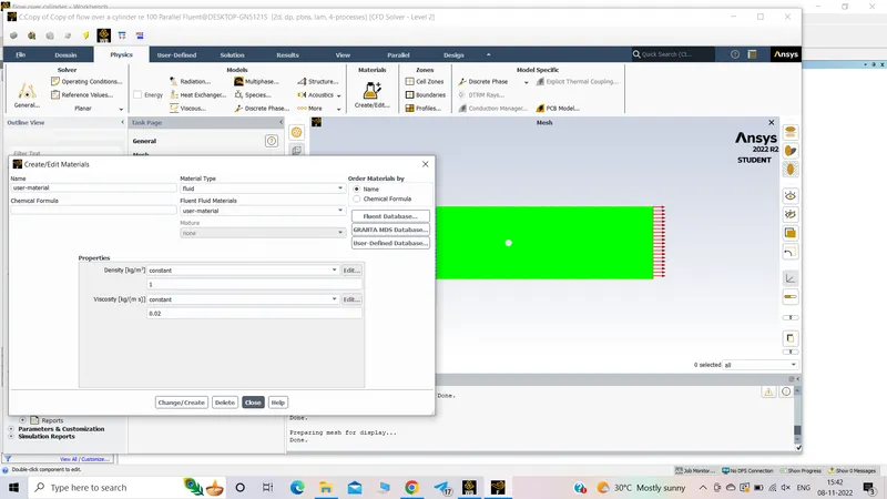
• creating user-material:

• Editing boundary condition:
• Edit velocity inlet:

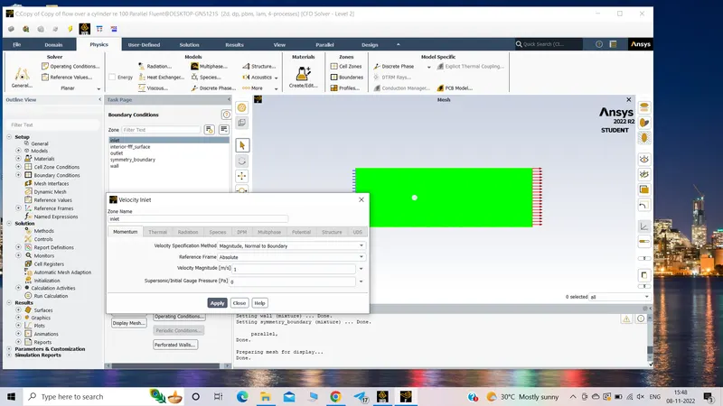
• To check the vortex nature it is important to know the Reynolds no.

The Reynolds number is a measure of the ratio of inertial to viscous forces in the flow of a fluid and may be defined as:

`Re=(rho*v*D)/(mu)`

`rho`=density

`v`=the steady velocity of the flow upstream of the cylinder

`D`=the diameter of the cylinder around which the fluid is flowing

`mu`=the kinematic viscosity of the fluid

`v=(Re*mu)/(rho.D)=(100*0.02)/(1*2)=1 (m/s)`

• Outlet- Pressure outlet
  Gauge Pressure- 0 Pa
• Symmetry- Symmetry
  Zone name- Symmetry
• Walls- Wall
  Wall motion- Stationary wall
  Shear condition- No slip

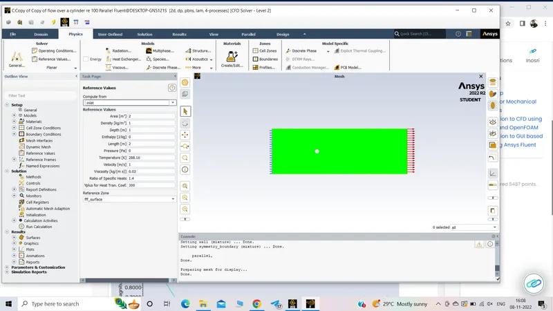
• setting reference value:

Monitor point set :

Report Definations

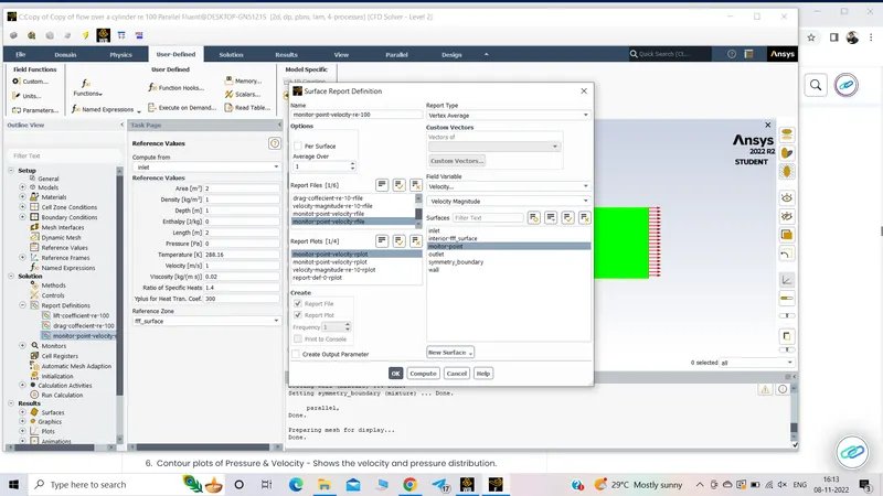
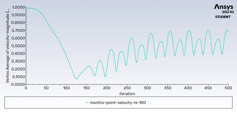
Create a Vertex average of velocity magnitude using surface report at a monitor point 8m away from the center of the cylinder to the right of the cylinder along X-direction.

Report defination to see monitor point velocity,drag coefficient and lift coefficient:

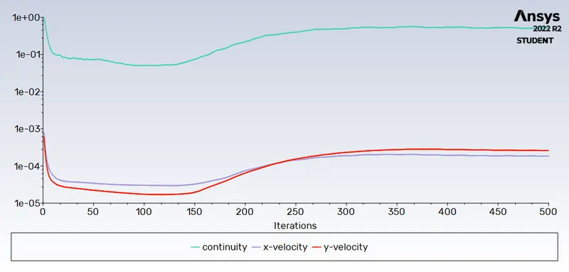
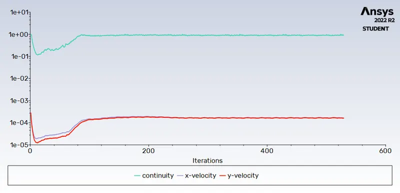
• Residual plot - This plot helps us in knowing at what point convergence is achieved.

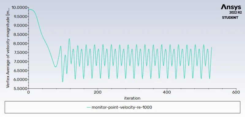
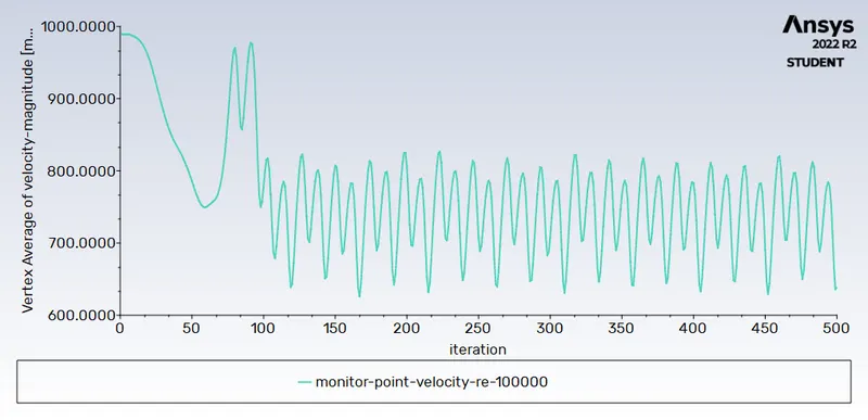
• Monitor point velocity plot - A monitor point is placed at a distance of 8m from the cylinder in order to calclate the velocity at that point

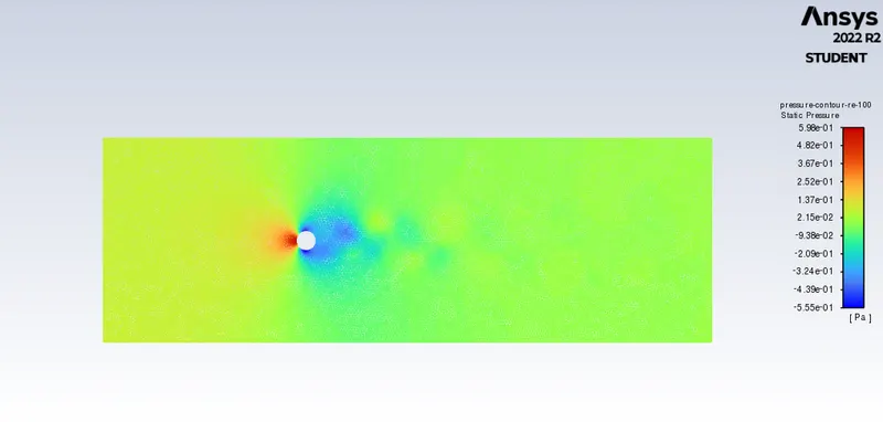
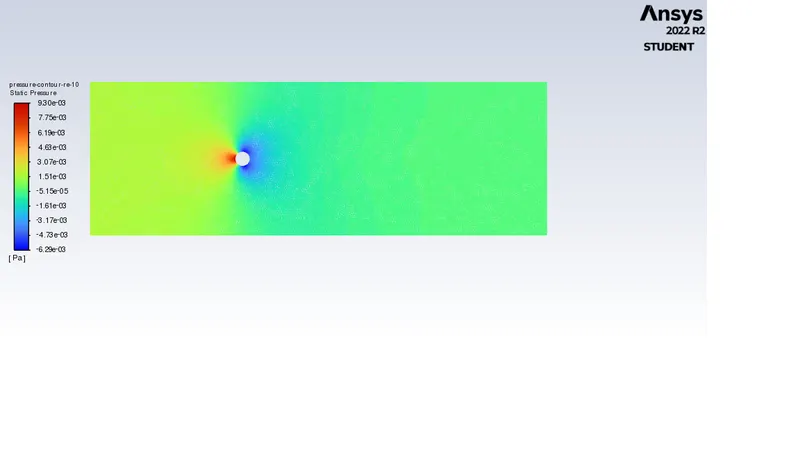
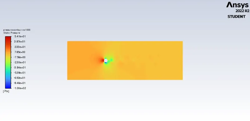
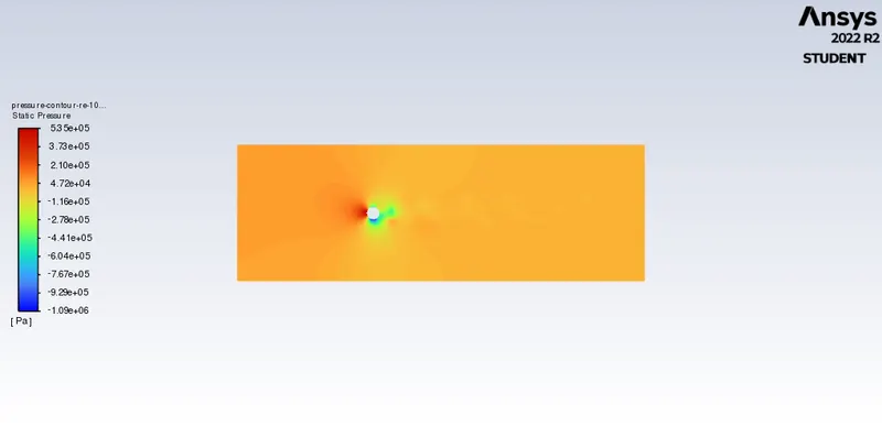
• Pressure contour plot - To see the pressure distribution

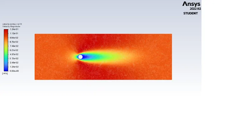
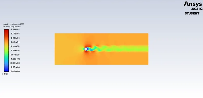
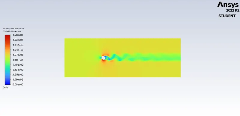
• Velocity contour plot - To see the velocity changes in the flow over the cylinder.

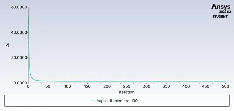
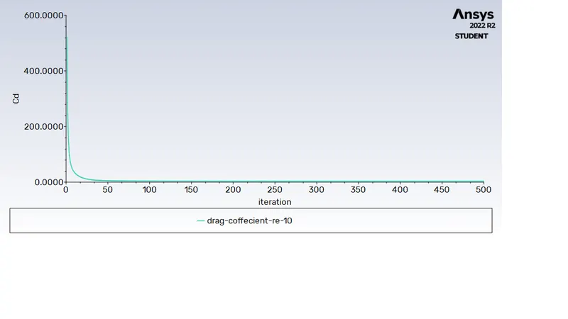
• Drag coefficient plot - To calculate the drag coefficient.

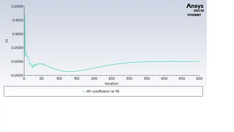
• Lift coefficient plot - To calculate the lift coefficient.

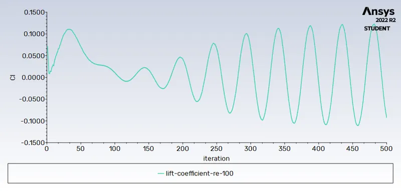
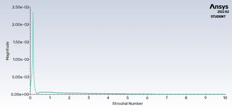
• Calculation of the Strouhal Number

Strouhal number is a dimensionless number describing oscillating flow mechanisms.

`St=(omega l)/v`

where

St = Strouhal Number

ω = oscillation frequency

l = characteristic length

v = flow velocity

Here,we have calculated staruhal no.using ansys fluent.

1.Go to fluent solver > results > fft analyser > load lift coefficient file > select plot FFT

Here, x axis denotes strauhal number and y axis denotes magnitude.

2.To get the magnitude of strauhal number,

go to results > fft analyser > click on write fft to file > click on write fft.

Open the file in excel and 1st coloumn denotes the frequncy and 2nd coloumn denotes strauhal number.use the command max and select 2nd row and find the magnitude of strauhal number.

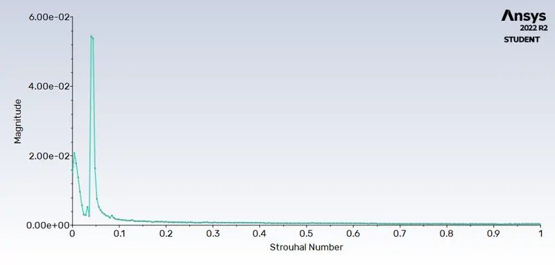
Strouhal number=0.043

• UnSteady case for Re= 100. (Part-I)

• Setting the solver: time:transient
• Method:standard
• No. of time step=600
• Time step size=0.1 sec

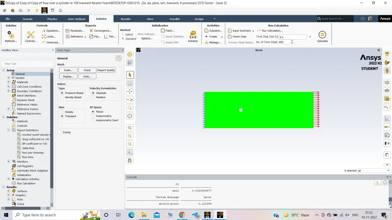
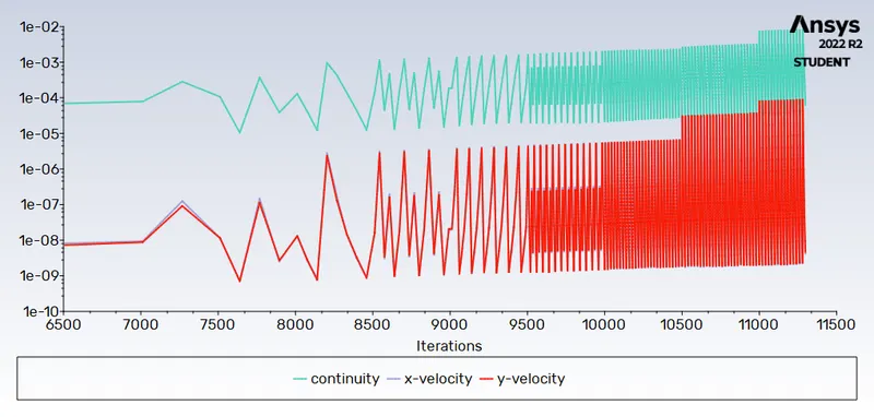
• Residual plot - This plot helps us in knowing at what point convergence is achieved.

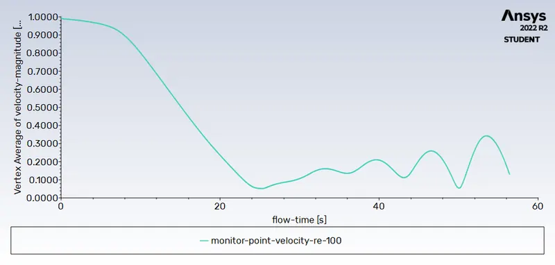
• Monitor point velocity plot - A monitor point is placed at a distance of 8m from the cylinder in order to calclate the velocity at that point

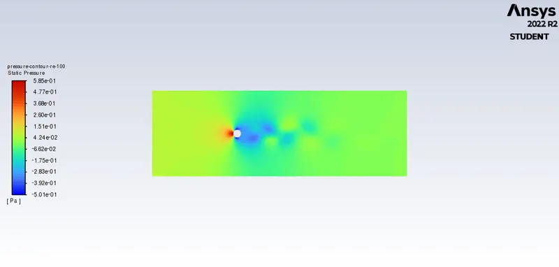
• Pressure contour plot - To see the pressure distribution

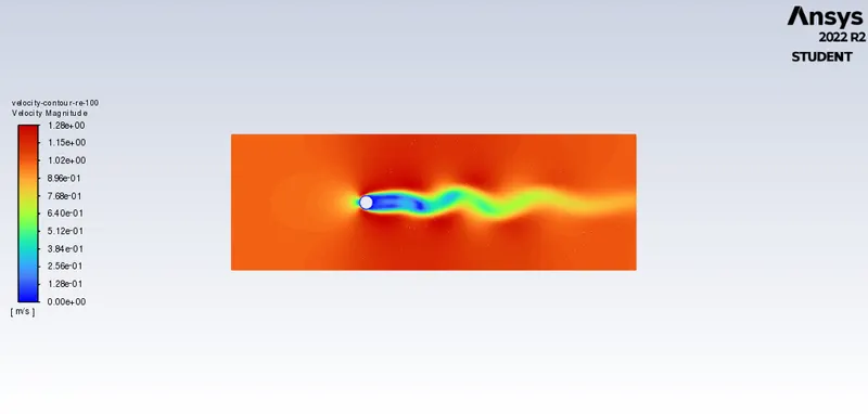
• Velocity contour plot - To see the velocity changes in the flow over the cylinder.

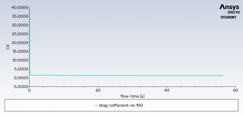
• Drag coefficient plot - To calculate the drag coefficient.

• Lift coefficient plot - To calculate the lift coefficient.

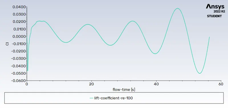
• Calculation of the Strouhal Number(=0.152)

• Steady case for Re= 10. (Part-II)

`v=(Re*mu)/(rho.D)=(10*0.02)/(1*2)=0.1 (m/s)`

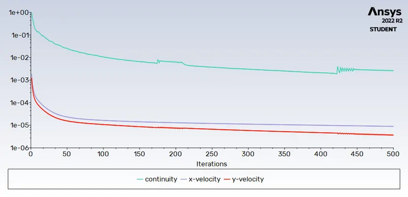
• Residual plot - This plot helps us in knowing at what point convergence is achieved.

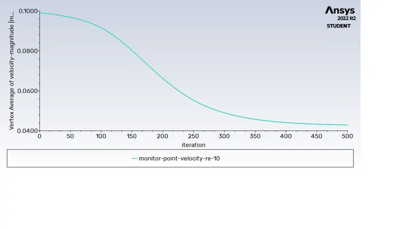
• Monitor point velocity plot - A monitor point is placed at a distance of 8m from the cylinder in order to calclate the velocity at that point

• Pressure contour plot - To see the pressure distribution

• Velocity contour plot - To see the velocity changes in the flow over the cylinder.

• Drag coefficient plot - To calculate the drag coefficient.

• Lift coefficient plot - To calculate the lift coefficient.

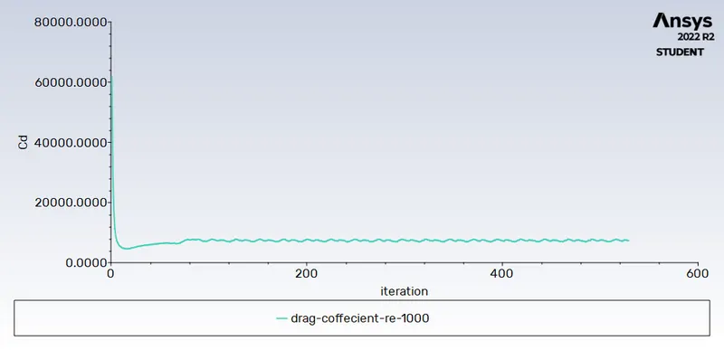
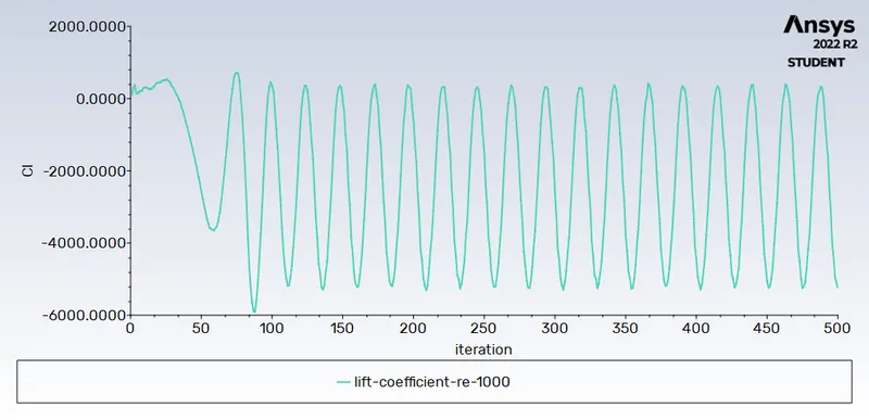
• Steady case for Re= 1000. (Part-II)

`v=(Re*mu)/(rho.D)=(1000*0.02)/(1*2)=10 (m/s)`

• Residual plot - This plot helps us in knowing at what point convergence is achieved.

• Monitor point velocity plot - A monitor point is placed at a distance of 8m from the cylinder in order to calclate the velocity at that point

• Pressure contour plot - To see the pressure distribution

• Velocity contour plot - To see the velocity changes in the flow over the cylinder.

• Drag coefficient plot - To calculate the drag coefficient.

• Lift coefficient plot - To calculate the lift coefficient.

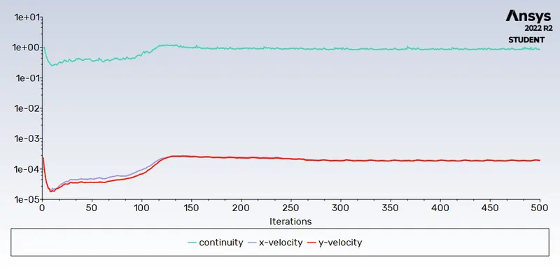
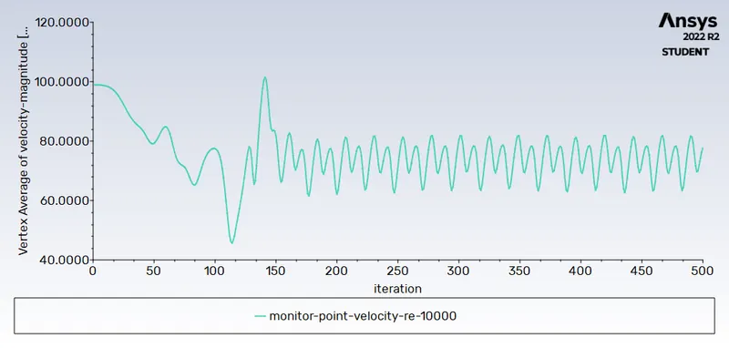
• Steady case for Re= 10000. (Part-II)

`v=(Re*mu)/(rho.D)=(10000*0.02)/(1*2)=100 (m/s)`

• Residual plot - This plot helps us in knowing at what point convergence is achieved.

• Monitor point velocity plot - A monitor point is placed at a distance of 8m from the cylinder in order to calclate the velocity at that point

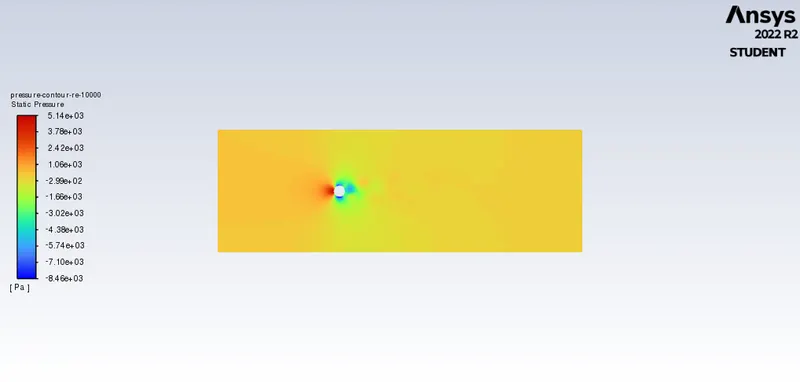
• Pressure contour plot - To see the pressure distribution

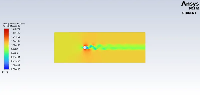
• Velocity contour plot - To see the velocity changes in the flow over the cylinder.

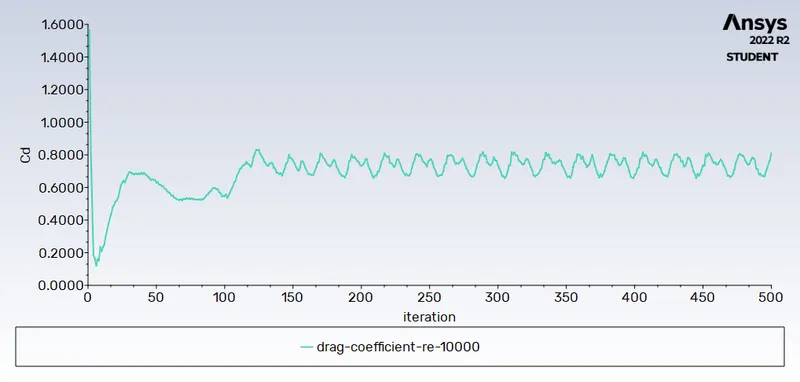
• Drag coefficient plot - To calculate the drag coefficient.

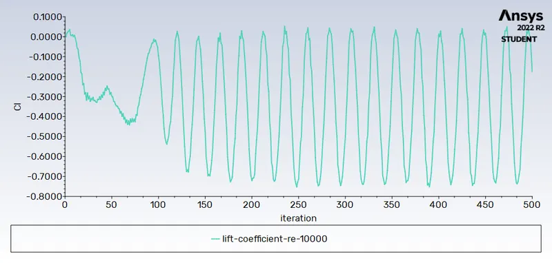
• Lift coefficient plot - To calculate the lift coefficient.

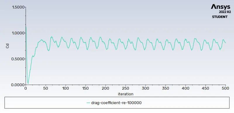
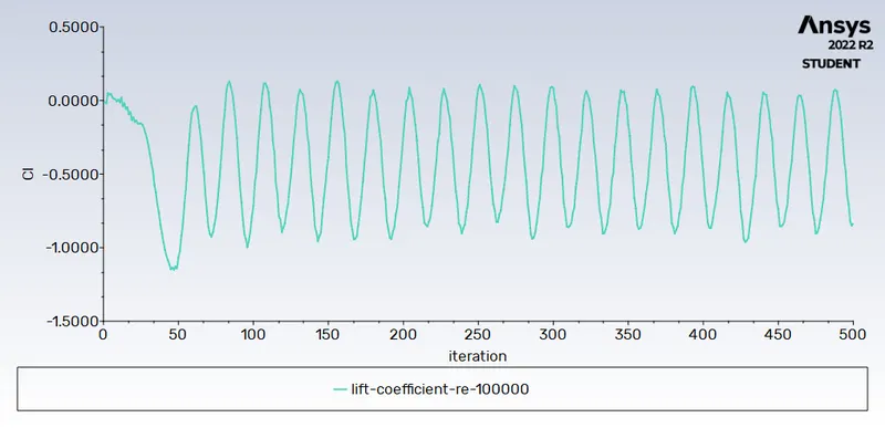
• Steady case for Re= 100000. (Part-II)

`v=(Re*mu)/(rho.D)=(100000*0.02)/(1*2)=1000 (m/s)`

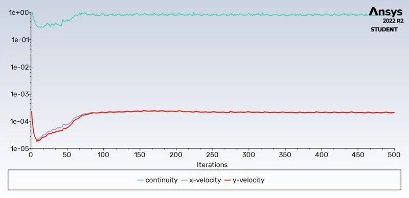
• Residual plot - This plot helps us in knowing at what point convergence is achieved.

• Monitor point velocity plot - A monitor point is placed at a distance of 8m from the cylinder in order to calclate the velocity at that point

• Pressure contour plot - To see the pressure distribution

• Velocity contour plot - To see the velocity changes in the flow over the cylinder.

• Drag coefficient plot - To calculate the drag coefficient.

• Lift coefficient plot - To calculate the lift coefficient.

Results:Values of coefficient of drag and lift coefficient for respective reynolds number is tabulated as follows:

Reynolds no	cd	cl
10(steady)	3.3269398	0.00012524896
100(steady)	1.3279219	-0.092175769
100(unsteady)	1.2789021	0.0020894977
1000(steady)	0.74571874	-0.526137
10000(steady)	0.81043017	-0.17528918
100000(steady)	0.81162566	-0.83557185

The effect of Reynolds number on the coefficient of drag:

When Reynolds number get increased the surface friction between fluid and cylinder is also increasing which casue the boundary layer to break before flow seperated hence amount of drag get decreases and lift get increases.As the Reynolds number increase in value, the wake region behind the cylinder is also increasing which results in bigger domain capturization for further simulations.For lower Reynolds number the vortices are bit symmetrical in nature but as Reynolds number get increase it start to deviate more.

Result validation:

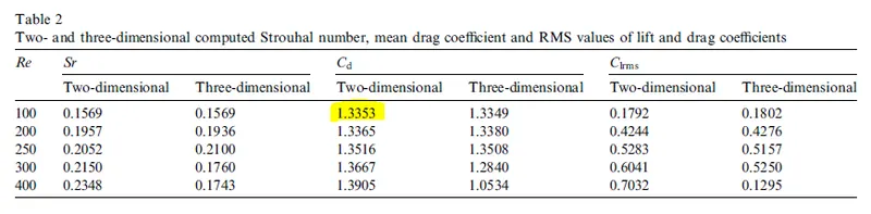
Calulated Cd for Re =100 is 1.3279 (steady) and 1.2789 (unsteady)which is nearly close to 1.3353 reference value.

Conclusion:

It is seen that the steady state solver is more time friendly compared with transient one but Non-iterative Time Advance method can provide better opportunity to solve same trasient problem with less number iteration and time also.

References:

References:

1.https://www.engineeringtoolbox.com/strouhal-number-d_582.html

2.https://www.sciencedirect.com/science/article/pii/S0307904X08000243

3. https://en.wikipedia.org/wiki/K%C3%A1rm%C3%A1n_vortex_street