Week 2 - Flow over a Cylinder.
Aim: - To simulate the flow over a cylinder and explain the phenomenon of Karman vortex street.
Objective: -
- To setup case for steady and transient simulation.
- To calculate the coefficient of drag and lift over a cylinder by setting different Reynolds numbers.
- To observe the effect of Reynolds number on coefficient of drag.
- To calculate the Strouhal number.
Theory
Vortex shadding:
vortex shedding is an oscillating flow that takes place when a fluid such as air or water flows past a bluff (as opposed to streamlined) body at certain velocities, depending on the size and shape of the body. In this flow, vortices are created at the back of the body and detach periodically from either side of the body forming a Von Karman vortex street. The fluid flow past the object creates alternating low-pressure vortices on the downstream side of the object. The object will tend to move toward the low-pressure zone.
If the bluff structure is not mounted rigidly and the frequency of vortex shedding matches the resonance frequency of the structure, then the structure can begin to resonate, vibrating with harmonic oscillations driven by the energy of the flow. This vibration is the cause for overhead power line wires humming in the wind, and for the fluttering of automobile whip radio antennas at some speeds. Tall chimneys constructed of thin-walled steel tubes can be sufficiently flexible that, in air flow with a speed in the critical range, vortex shedding can drive the chimney into violent oscillations that can damage or destroy the chimney.
A very interesting sequence of events begins to develop when the Reynolds number is increased beyond 40, at which the wake behind the cylinder becomes unstable. The wakes develop a slow oscillation in which the velocity is periodic in time and downstream direction. The oscillation wake rolls up into two staggered rows of vortices with opposite sense of rotation. And these rows form a street known as von Karman vortex street.
The Reynolds number is a key parameter in fluid dynamics. It describes the fluid, geometry and flow. This allows us to compare different fluid system.
`Re=[ρvD]/μ`
`ρ=` density of fluid
V = in flow velocity
D = diameter of cylinder
`μ=` dynamic viscosity of fluid
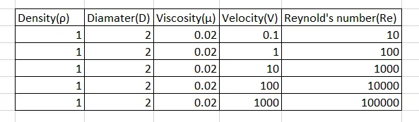
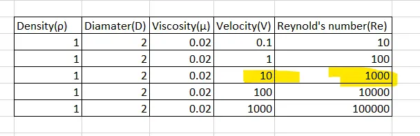
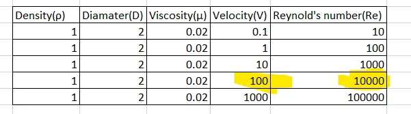
calculation of velocity for given Reynolds number in excel
solving and modelling approach
The main aim of the project is to study the behavior of Reynolds number on the flow over a cylinder. to capture the flow with every regime it is important to have more flow domain and less mesh size to capture every possible vortex in wake region.
The problem is divided into two group in which both steady and unsteady state simulation will be carried accordingly. In steady state simulation the varying Reynolds number will be taken into consideration by maintaining fluid property constant. The simulation will be running for 10, 100, 1000, 10000, 100000 Reynolds number and accordingly the other parameters will be studied. The problem will start with 2D geometry of flow field and mesh afterwards. It is important to have less mesh size to capture every little detail from flow domain. The inflation layer will be added near the cylinder wall to capture the boundary layer detachment from the surface of cylinder. The boundary conditions will be simple as velocity inlet and pressure outlet with symmetry wall type condition. The cylinder will be also considering as wall type in which coefficient of lift and drag will be calculated.
For steady state solver simple interpolation scheme will be used to calculate results in neighboring volume. Unsteady state simulation will also be done using the simple interpolation scheme. To check for convergence of solution. we will create some plots which have vertex average velocity 8m behind the cylinder which will be used to plot Strouhal number later using FFT option in FLUENT. after that lift coefficient and drag coefficient will be calculated on the cylinder wall.
The coefficient of drag and lift are the function of respective lift and drag force with density of fluid and velocity with exposure area in front. the equation for coefficient of lift and drag is given as:
`C_d=(2F_d)/(ρV^2 A)`
`C_l=(2F_l)/(ρV^2 A)`
`F_d` and `F_l` are drag and lift force respectively.
`rho` = density of fluid.
v = velocity of fluid
A = frontal area.
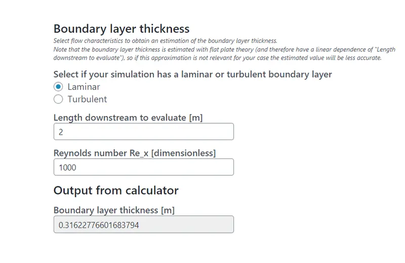
The inflation layer that I m adding in such a way that total inflation layer thickness should be greater than the boundary layer thickness.
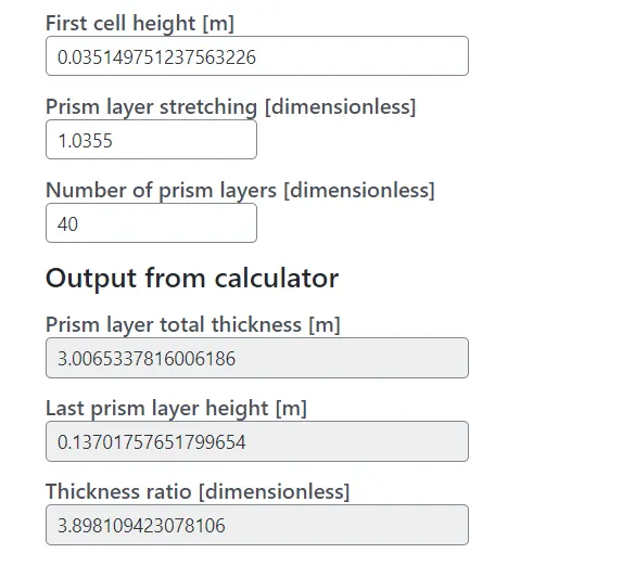
The first cell height is calculated from the assumed value of y+. The height of last layer in inflation layer should be equal to mesh length.
CASE SETUP FOR STEADY STATE
Geometry
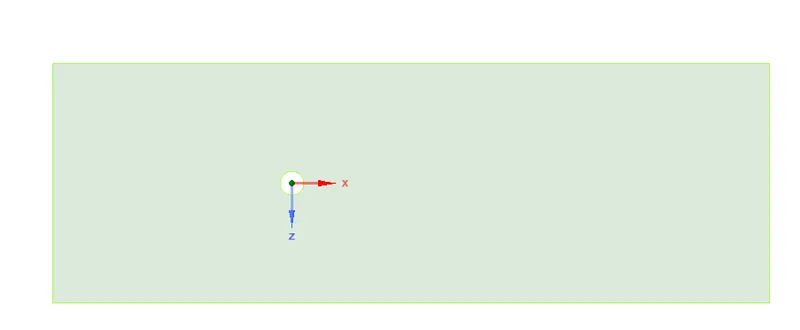
- firstly draw a 2m circle.
- draw a 20m line from the center of the circle to the left.
- draw a 10m long line in both upward and downward from the end of the line.
- draw a 40m line from the center of the circle to the right.
- now draw a rectangle from the left corner end to the right line end of dimension 20X40m.
- delete the line 1, 2, 3 and 4.
- now select the inner area of the circle we will get the desired surface.
Meshing
For meshing I m selecting different values of y+ for different Reynold's number.
For the first case, I m choosing y+ = 0.10 to generate mesh, because I get more orthogonal inflation layer around this y+ value.
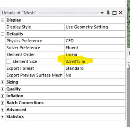
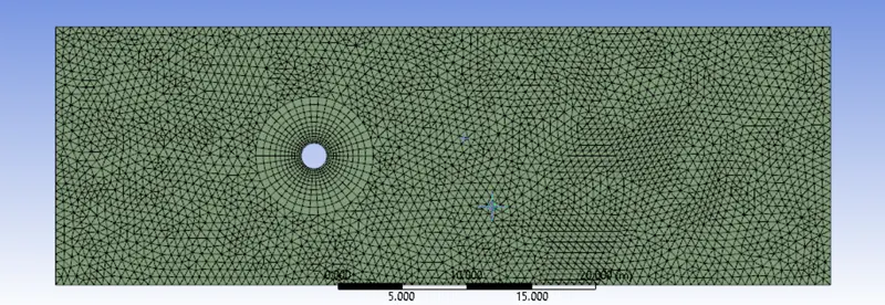
The mesh length is shown below
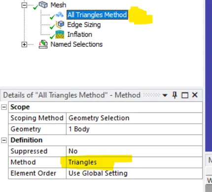
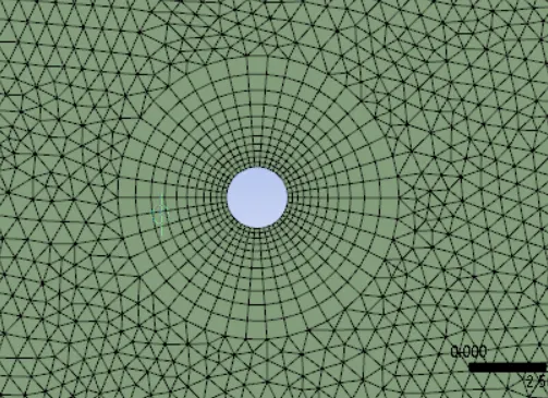
The mesh is inserted as triangle in shape
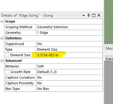
The edge sizing and inflation layer values are given same value to get inflation layer more orthogonal near the wall.
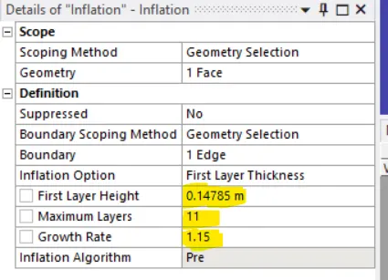
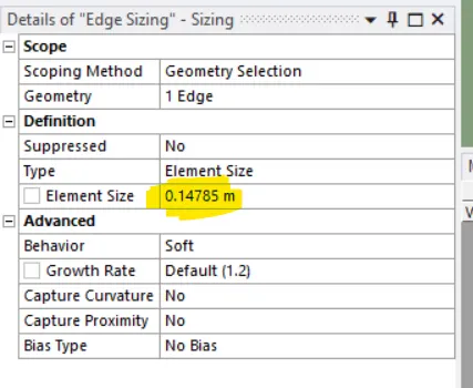
The calculation for first layer thickness is shown below.
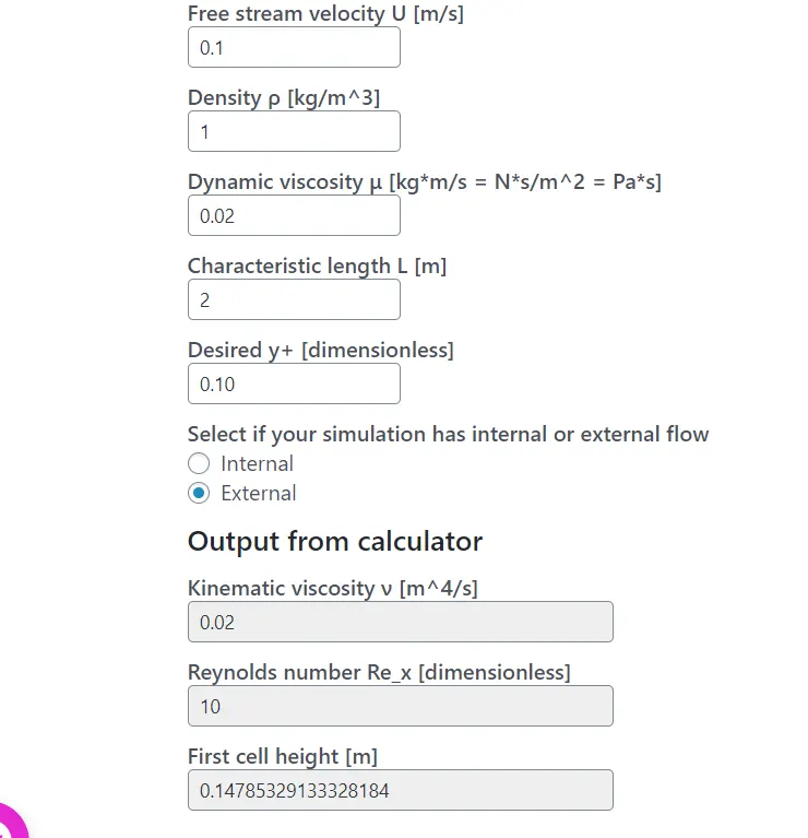
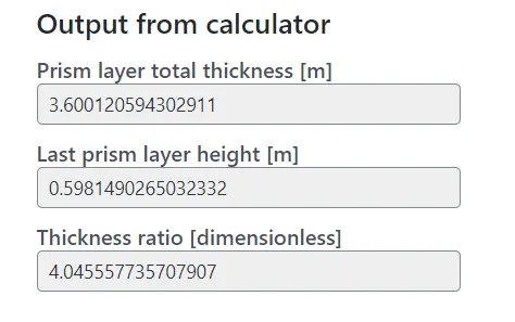
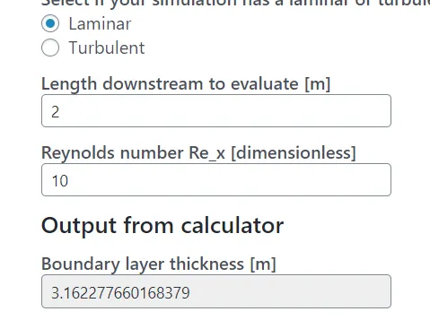
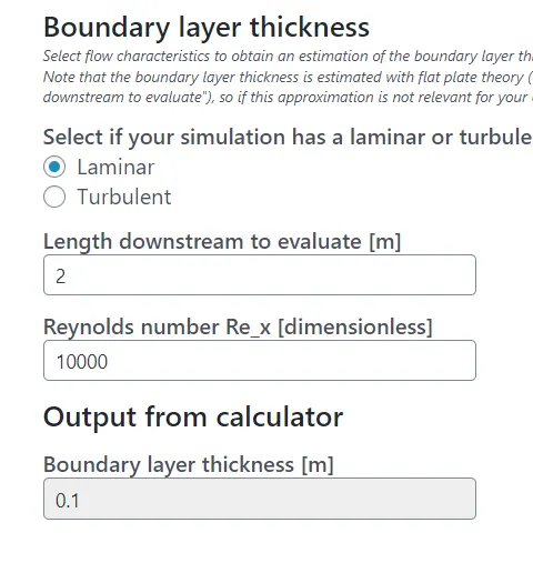
Here the boundary layer is 3.16 m. So, total prism layer thickness should be greater than 3.16 m. In this case, we got 3.60 m. So, we can move ahead.
After meshing, the mesh looks like this
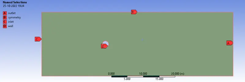
now assign the names for the boundaries.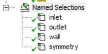
Setup
- after opening fluent setup select physics the go to general setting there we will select:
A. pressure based type.
B. absolute velocity formula
C. Steady state solver
D. planer 2D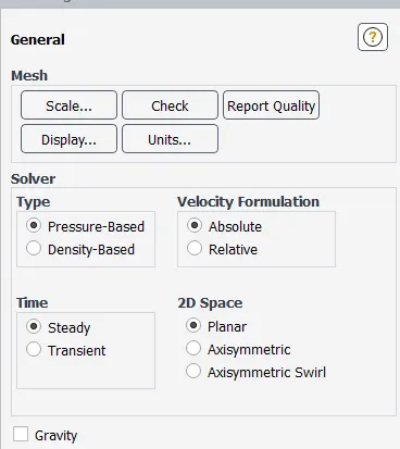
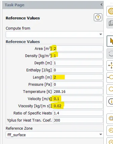
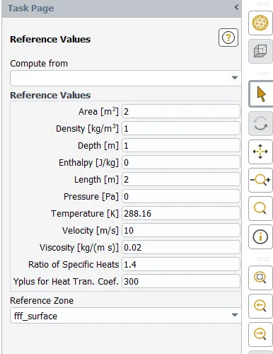
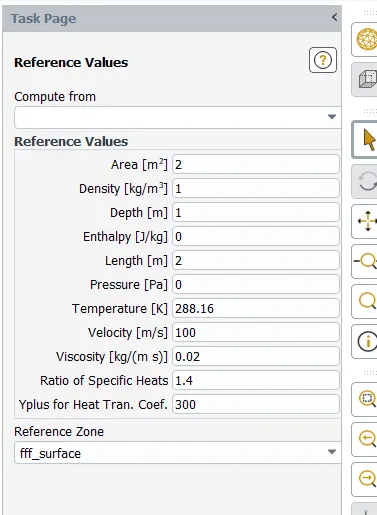
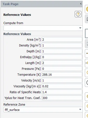
- change reference values as given below:
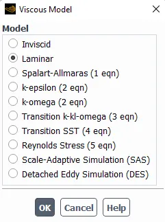
- change the turbulence model to laminar
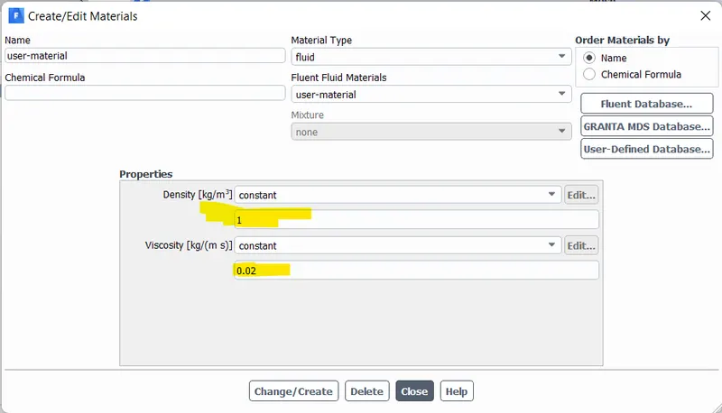
- select an edited user material of density `1Kg/m^3` and viscosity `0.02 Kg/m*s` of type fluid.
- change the boundary conditions.
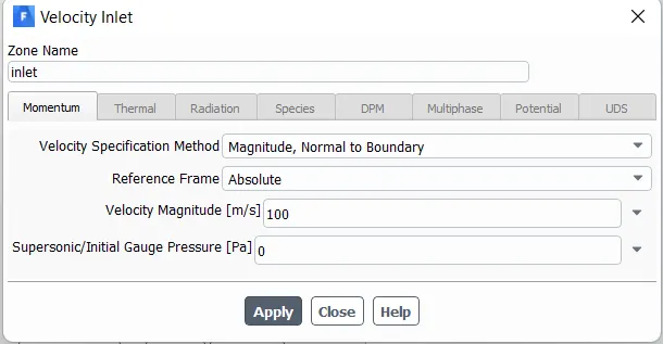
a. change the inlet velocity as calculated for particular Reynolds number.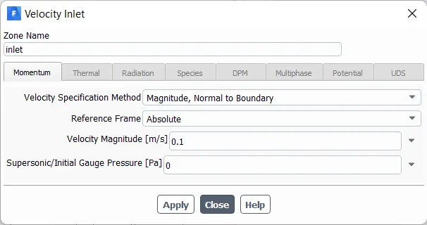
b. for outlet make sure the outlet is pressure outlet and it is set to zero pascal gauge pressure.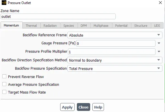
c. Check the wall is no slip and stationary wall
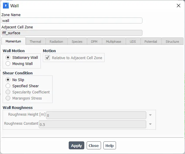
d. make sure that symmetry type is symmetry.
6.now change the solution method pressure velocity coupling to SIMPLE.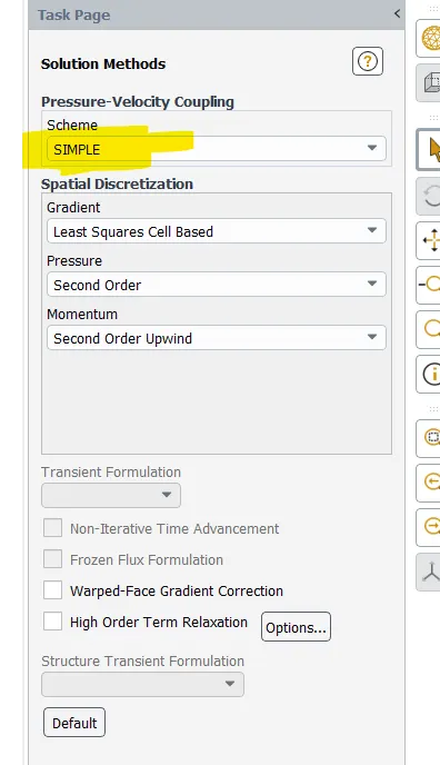
1.Now add report definition for drag and lift coefficient 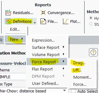
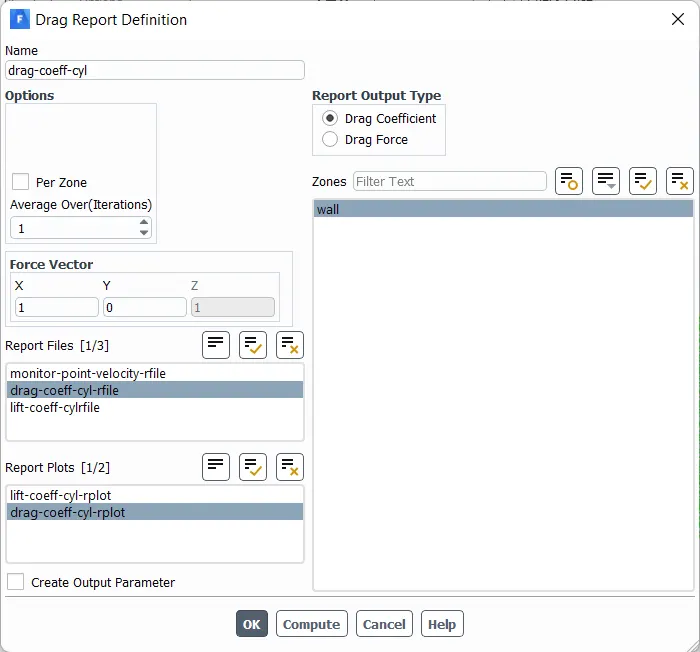
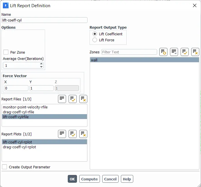
2.from results section create a point 'monitor point' 8m away from the center of the circle in x-direction.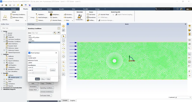
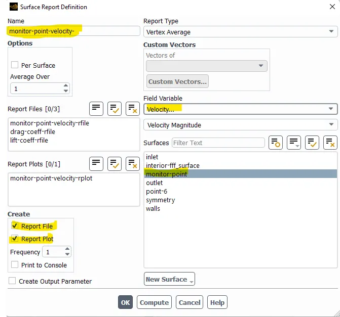
3.Now create a report definition at monitor point for vertex average velocity.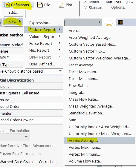
change name => change field variable to velocity=>select monitor point
4.now initialize the solution with hybrid initialization type.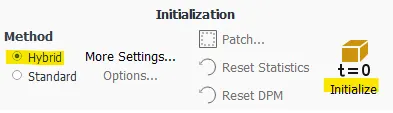
5.From results section create pressure and velocity contour.
result=>graphics=>contour=>new
6.change contour name and variable then select all surfaces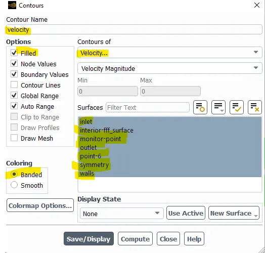
7.Open residuals then uncheck convergence so that solution will not stop after converging automatically.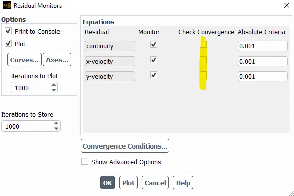
8.Now run the simulation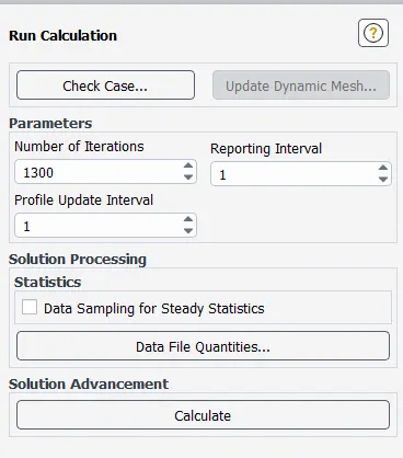
Output from the simulation
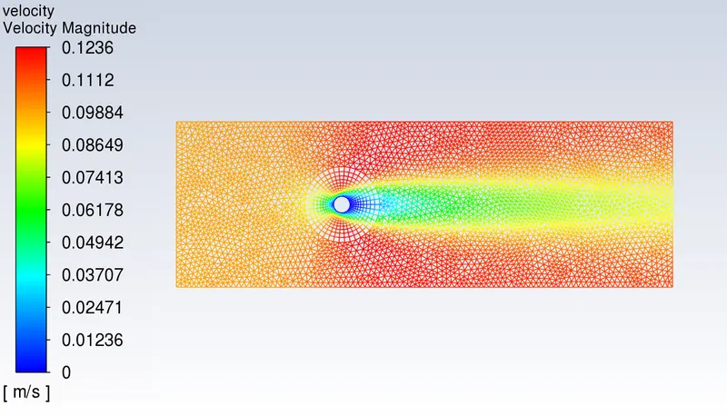
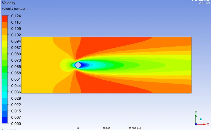
1)Here I m plotting the output when Re=10
Velocity contour (Re=10)
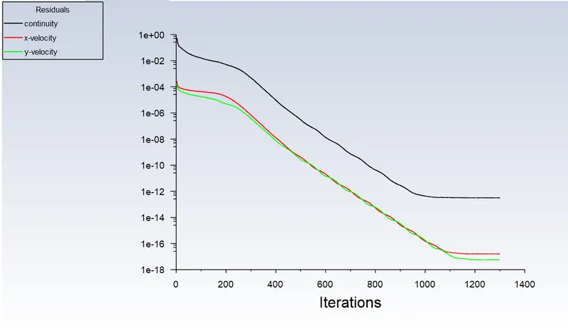
Residuals
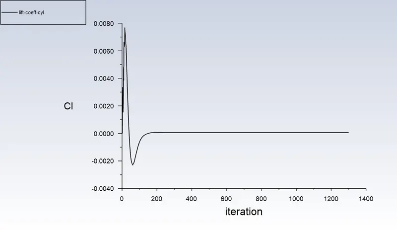
Coefficient of lift
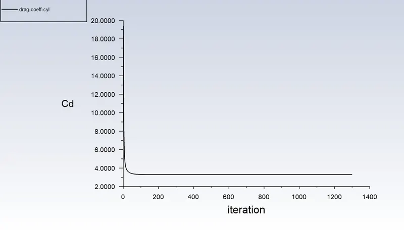
Coefficient of drag
Monitor point velocity
Convergence
By looking at residuals plot for lower Reynolds number, we can say that solution has converged, because we can observe that it is almost linear towards the end of the iteration.
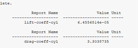
Coefficient of lift = 6.4556814e-05.
Coefficient of drag = 3.3038735.
By comparing the coefficient of drag with standard literature, we can say that I got the correct value for drag coefficient.
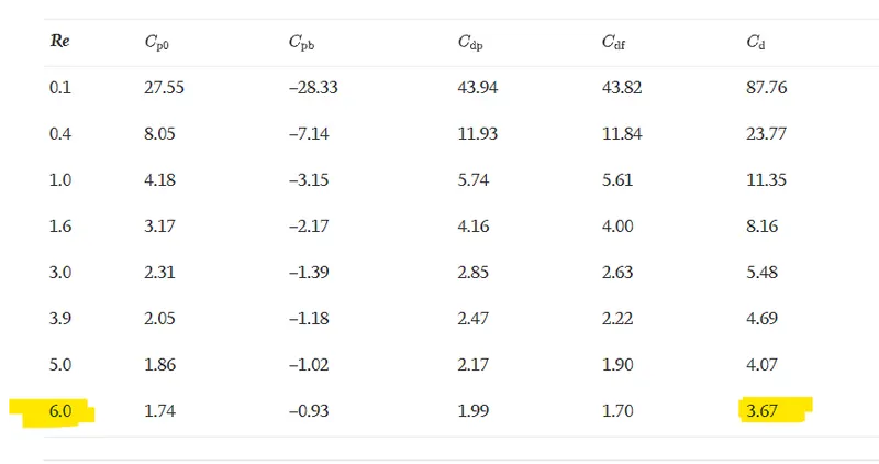
In literature, they mentioned Cd=3.67, when Re=6.
But for me, Cd=3.3038735, when Re=10.
So, I think that I got the right value for Cd.
Vertex average velocity
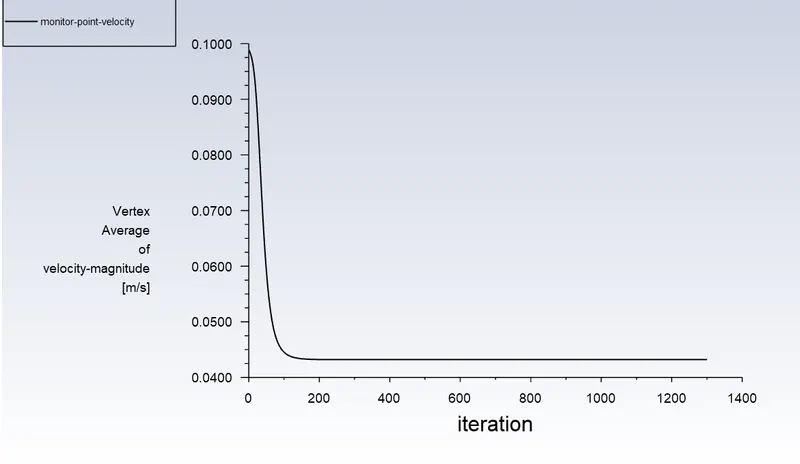
At Re=10, there is no vortex shedding.
At this Re,laminar flow (L2) with steady separation (4<Re<48">(4<Re<48) forming a symmetric contra-rotating pair of vortices in the near wake.
So, the vertex average is constant and the value is converged to 0.04320487 [m/s].
2) Moving for mesh generation and plotting for Re=1000
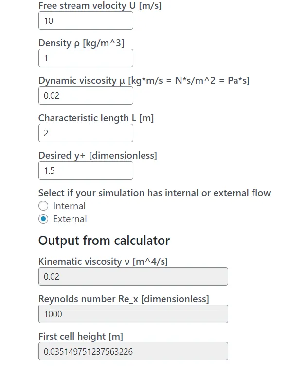
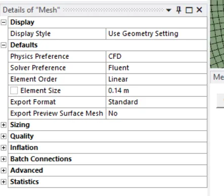
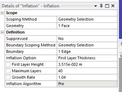
Here I select y+ = 1.5, So, the first cell height and mesh size are shown below. I m going for mesh length of 0.25 m in order to make save the computational cost. So, I prfer more number of inflation layer to make it orthogonal. The growth rate that is suitable for orthogonal is 1.04.
The calculation is shown below
The values that I put to generate mesh is shown below
Inflation layer
Edge sizing
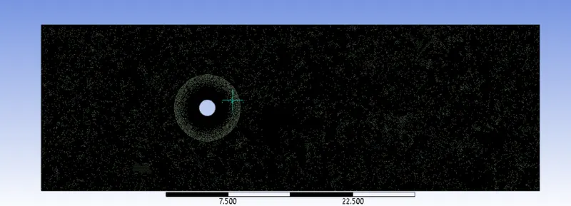
The final generated mesh is shown below
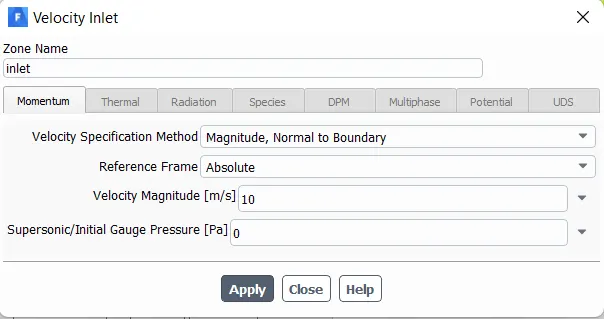
Perform all other operations to make velocity as 10 m/s in set up. This is similar to what we done with Re=10.
Start simulation
Output from the simulation
1)Here I m plotting the output when Re=1000
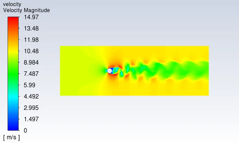
Velocity contour (Re=1000)
Residuals
Coefficient of lift
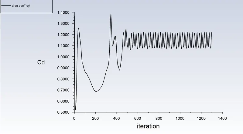
Coefficient of drag
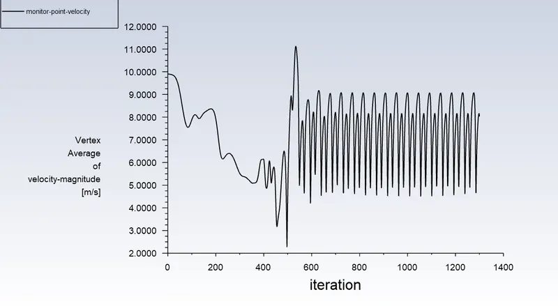
Monitor point velocity
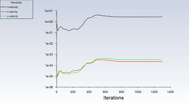
Convergence
By looking at residuals plot for lower Reynolds number, we can say that solution has converged, because we can observe that it is almost linear towards the end of the iteration.
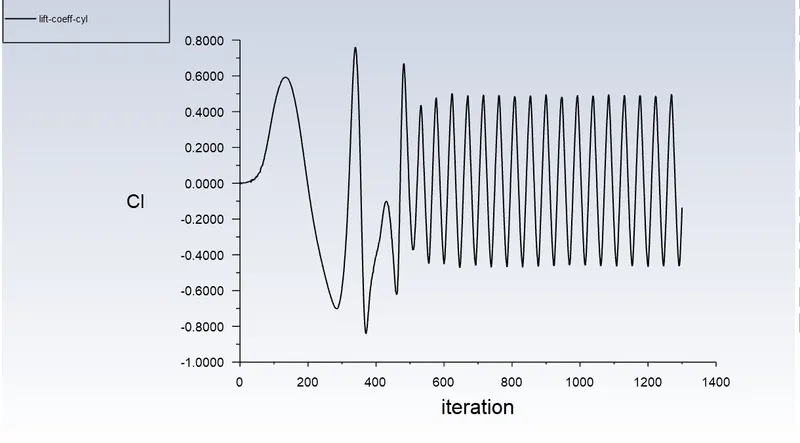
Coefficient of lift = Oscilating between -0.5 to 0.5.
Coefficient of drag = Oscilating between 1.08 to 1.22.
By comparing the coefficient of drag with standard literature, we can say that I got the correct value for drag coefficient.
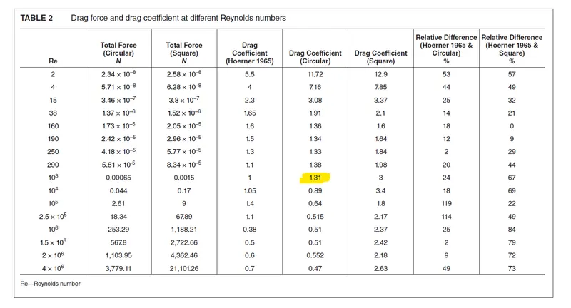
In literature, they mentioned Cd=1.31, when Re=1000.
But for me, Cd is oscilating between 1.08 to 1.22, when Re=1000. There is small variation in Cd because in journal they used K-Omega SST model with rectangular mesh.
Vertex average velocity
At Re=1000, there is vortex shedding.
Values are oscilating between 4.5 to 9 m/s.
The animation video is attached below
3) Moving for mesh generation and plotting for Re=10000
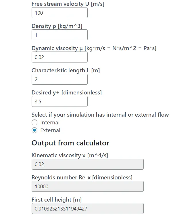
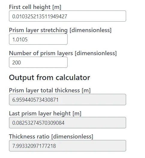
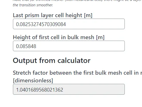
Here I select y+ = 3.5, So, the first cell height and mesh size are shown below. I m going for mesh length of 0.085848 m in order to make save the computational cost. So, I prfer more number of inflation layer to make it orthogonal. The growth rate that is suitable for orthogonal is 1.0105.
The calculation is shown below
The values that I put to generate mesh is shown below
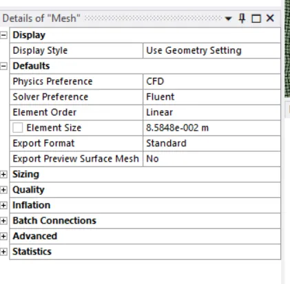
Inflation layer
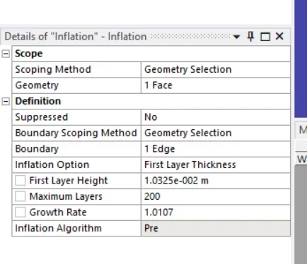
Edge sizing
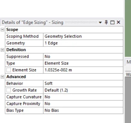
The final generated mesh is shown below
Perform all other operations to make velocity as 100 m/s in set up. This is similar to what we done with Re=10.
*****************************************************************************************************************************
Start simulation
Output from the simulation
1)Here I m plotting the output when Re=10000
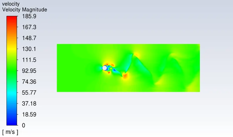
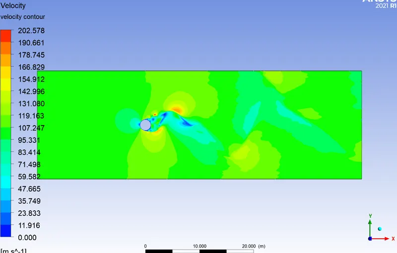
Velocity contour (Re=10000)
Residuals
Coefficient of lift
Coefficient of drag
Monitor point velocity
Convergence
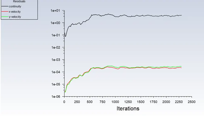
By looking at residuals plot for lower Reynolds number, we can say that solution has converged, because we can observe that it is almost linear towards the end of the iteration.
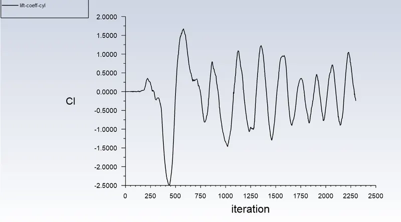
Coefficient of lift = Oscilating between around -1 to 1.
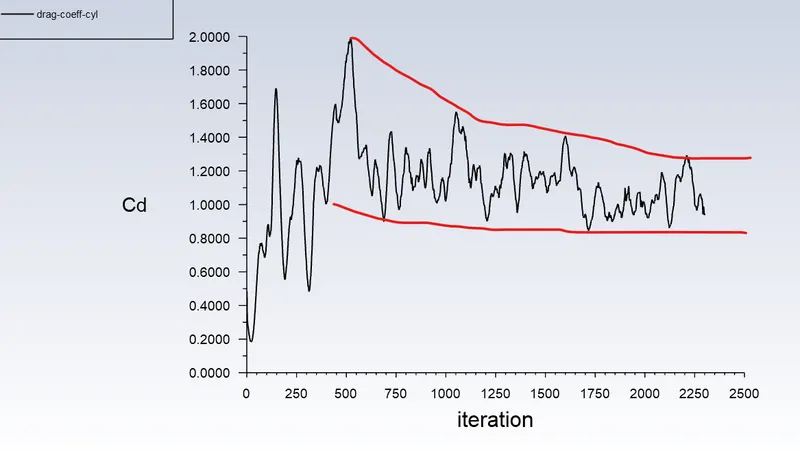
Coefficient of drag = Oscilating between 0.95 to 1.40.
By comparing the coefficient of drag with standard literature, we can say that I got the correct value for drag coefficient.
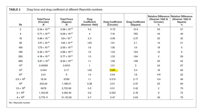
In literature, they mentioned Cd=0.89, when Re=10000.
But for me, Cd is oscilating between 0.95 to 1.40, when Re=10000. There is small variation in Cd because in journal they used K-Omega SST model with rectangular mesh.
Vertex average velocity
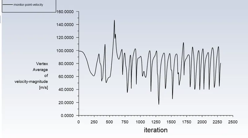
At Re=10000, there is vortex shedding.
Values are oscilating between 50 to 110 m/s.
4) Moving for mesh generation and plotting for Re=100000
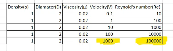
Here I m simply adding inflation layer without looking y+ values and using quad elements for meshing.
The meshing parameters are shown below
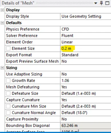
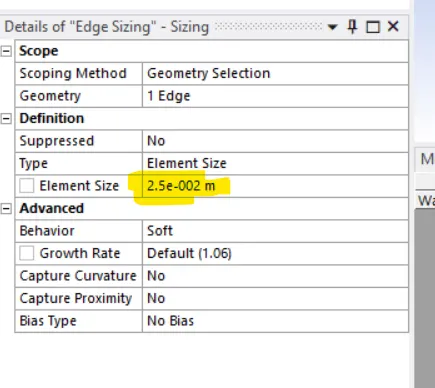
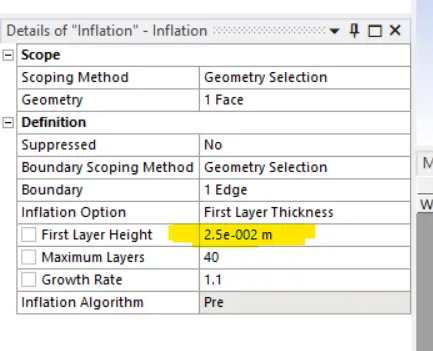
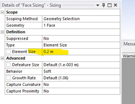
Do all other things such that the inlet velocity is set to 1000 m/s such that Re=100000.
Start simulation
Output from the simulation
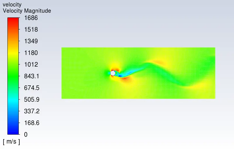
Here I m plotting the output when Re=100000
Velocity contour (Re=100000)
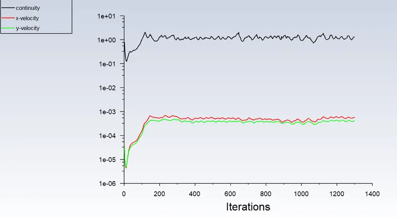
Residuals
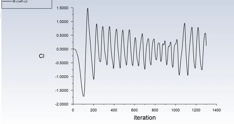
Coefficient of lift
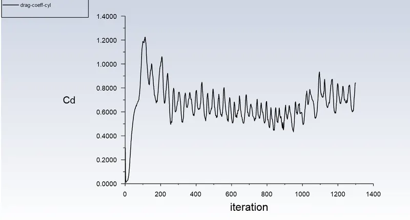
Coefficient of drag
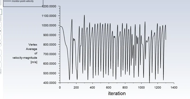
Monitor point velocity
Convergence
By looking at residuals plot for lower Reynolds number, we can say that solution has converged, because we can observe that it is almost linear towards the end of the iteration and there is some wave nature in scaled residual graph.
Coefficient of lift = Oscilating between around -0.75 to 0.75 towards the end of iteration
Coefficient of drag = Oscilating between 0.60 to 0.90 towards the end of iteration
By comparing the coefficient of drag with standard literature, we can say that I got the correct value for drag coefficient.
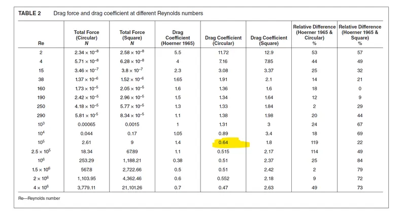
In literature, they mentioned Cd=0.64, when Re=100000.
But for me, Cd is oscilating between 0.60 to 0.90, when Re=100000. There is small variation in Cd because in journal they used K-Omega SST model with rectangular mesh.
Vertex average velocity
At Re=100000, there is vortex shedding.
Values are oscilating between 400 to 1000 m/s.
5) Moving for mesh generation and plotting for Re=100
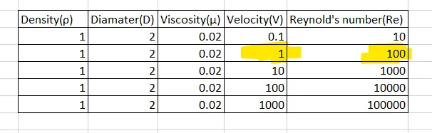
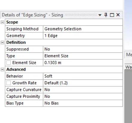
Here I select y+ = 0.7, So, the first cell height and mesh size are shown below. I m going for mesh length of 0.3072 m in order to make save the computational cost. So, I prfer more number of inflation layer to make it orthogonal. The growth rate that is suitable for orthogonal is 1.10.
The calculation is shown below
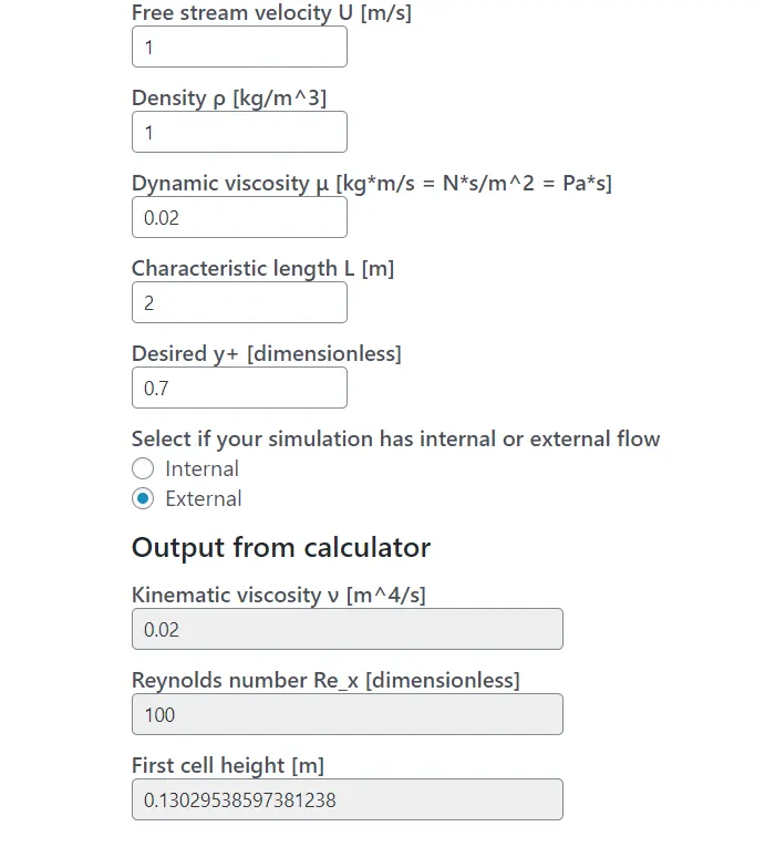
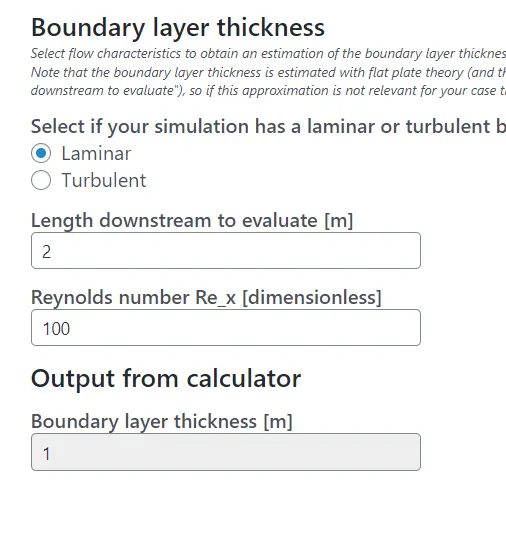
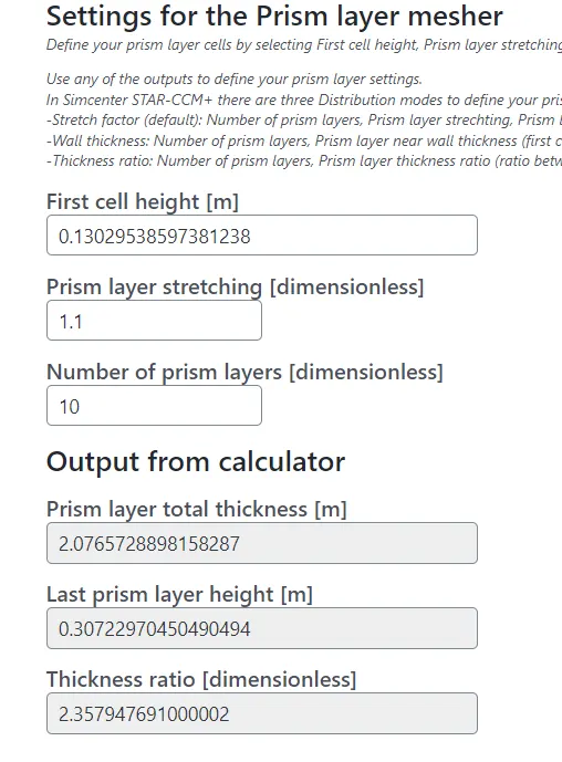
The values that I put to generate mesh is shown below
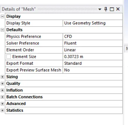
Inflation layer
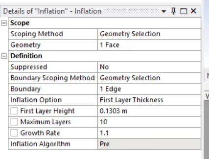
Edge sizing
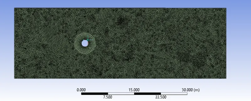
The final generated mesh is shown below
Perform all other operations to make velocity as 1 m/s in set up. This is similar to what we done with Re=10.
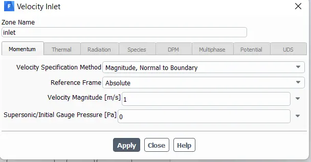
Start simulation
Output from the simulation
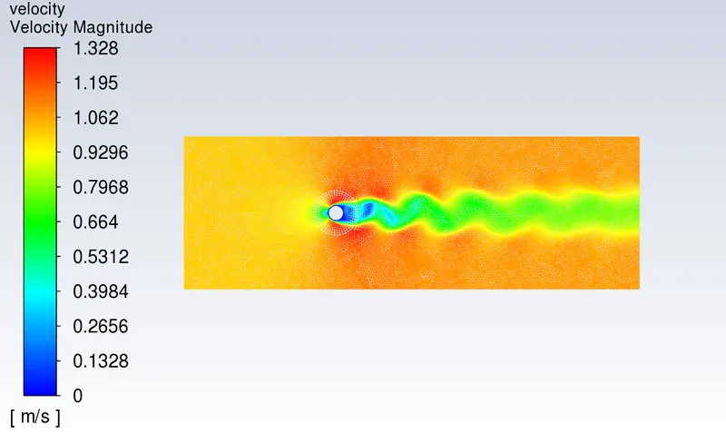
5)Here I m plotting the output when Re=100
Velocity contour (Re=100)
Residuals
Coefficient of lift
Coefficient of drag
Monitor point velocity
Convergence
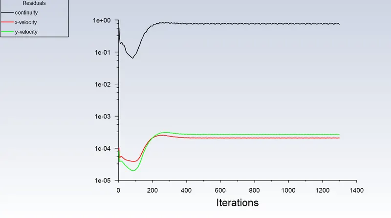
By looking at residuals plot for lower Reynolds number, we can say that solution has converged, because we can observe that it is almost linear towards the end of the iteration.
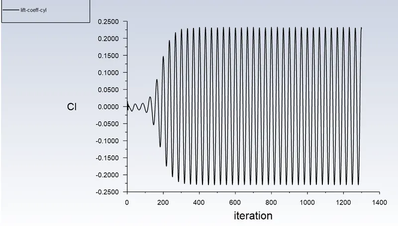
Coefficient of lift = Oscilating between around -0.23 to 0.23.
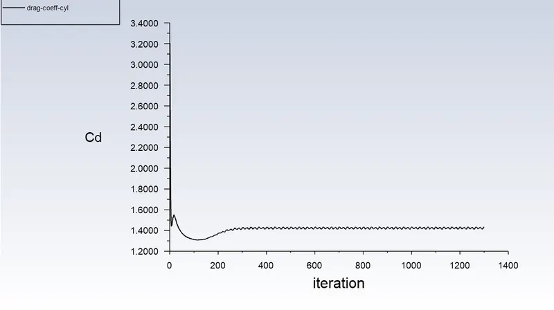
Coefficient of drag = Oscilating between 1.42 to 1.46.
By comparing the coefficient of drag with standard literature, we can say that I got the correct value for drag coefficient.
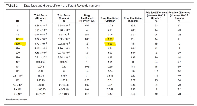
In literature, they found Cd=1.91, when Re=38 and Cd=1.36 when Re=160.
But for me, Cd is oscilating between 1.42 to 1.46, when Re=100. There is small variation in Cd because in journal they used K-Omega SST model with rectangular mesh.
So my value is almost correct
Vertex average velocity
At Re=100, there is vortex shedding.
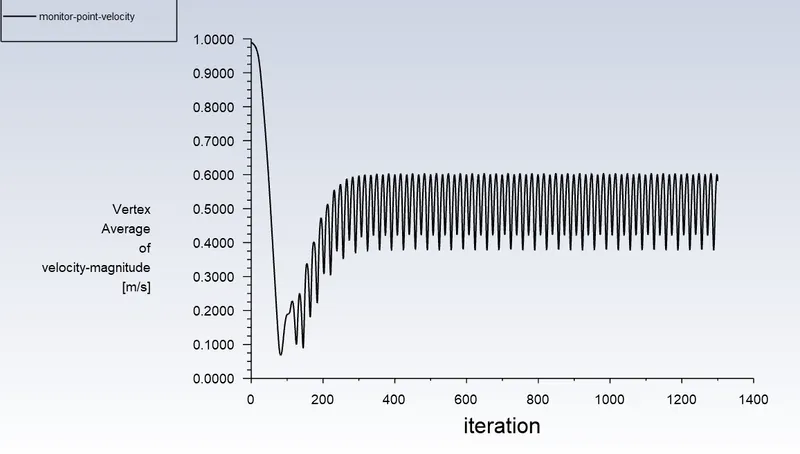
Values are oscilating between 0.38 to 0.62 m/s.
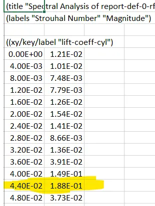
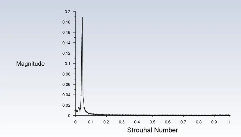
Strouhal number for Re=100
-----------------------------------------------------
CASE SETUP FOR TRANSIENT CASE
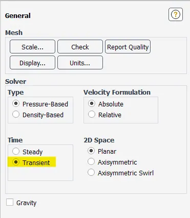
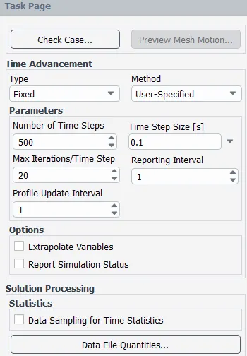
For transient case most of the steps are similar as steady state except
- Transient
- Solution run method
OUTPUT FOR TRANSIENT STATE SOLUTION
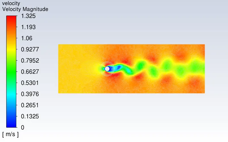
VELOCITY CONTOUR
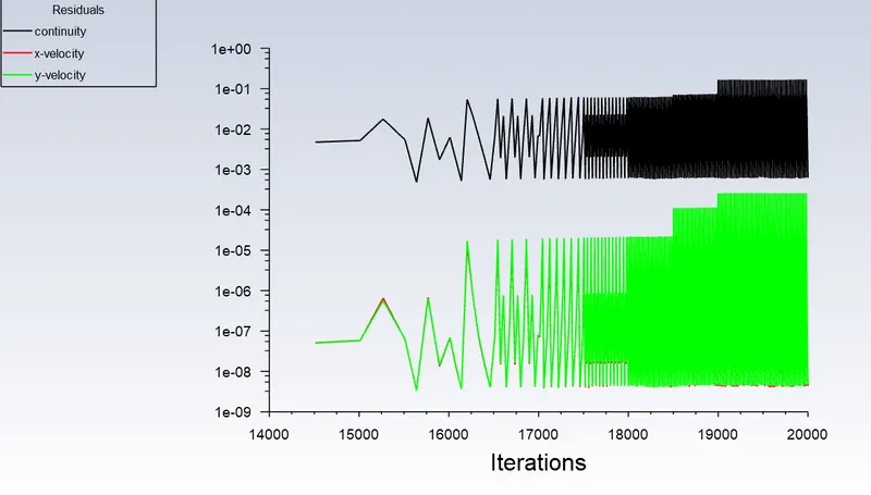
Residuals
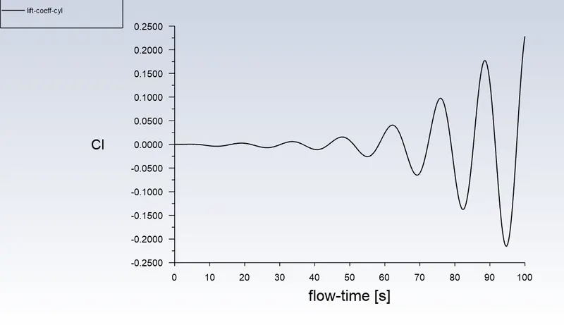
Coefficient of lift
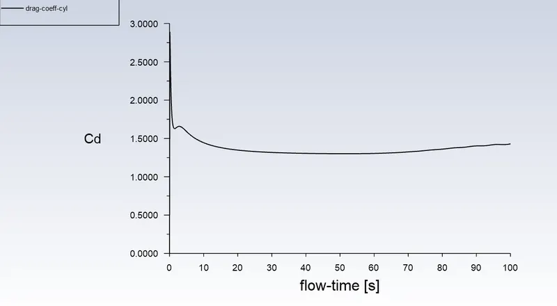
Coefficient of drag
Monitor point velocity
Convergence
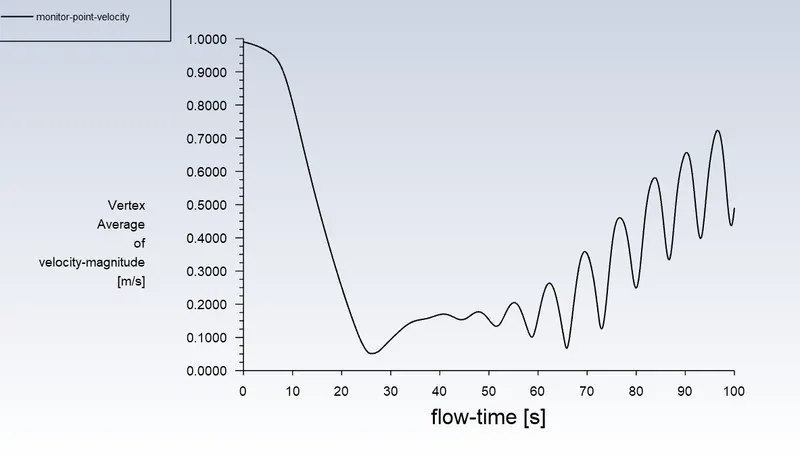
By looking at residuals plot for lower Reynolds number, we cannot say that solution has converged with the 1000 time steps, it needs to run more so as to converge, but due to storage capacity in laptop further more iteration is not possible. If the solution is converged, it will have constant amplitude of hills and valleys in every graph especially in scaled residual graph. If we run for more time step, the solution will converge
Coefficient of lift = Value doesn't rech steady state with constant amplitude for 1000 time step iteration.
Coefficient of drag = Value found around 1.4292214, which is satisfying.
Vertex average velocity
At Re=100, there is vortex shedding.
In order to get converged value, the solution needs to be run for more time step which is practically impossible with current processor.
For the value of coefficient of lift and vertex average to be converged, we need to get the oscilations in transient simulation same as that of steady state.
Strouhal number for Re=100
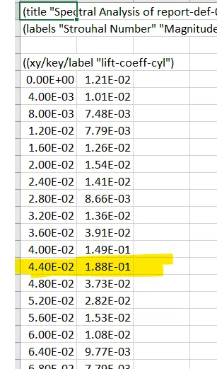
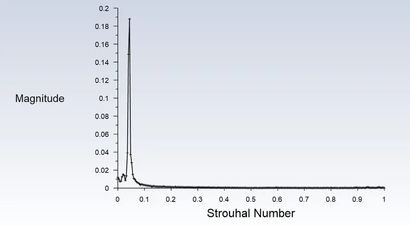
Got the same value of strouhal number magnitude in both transient and steady state simulations
Discuss the effect of Reynolds number on the coefficient of drag. [ Results should be validated with any standard literature and error should be within 5 %]
On increasing the Reynold's number the coefficient of drag of the cylinder reduces. The values are clearly compared with the standard literature results. The screenshot of the literature is also attached above while comparing the results.
If there is any variation, it is due to the methods they adopted in the literature. In literature, the professors MEHMET ISHAK YUCE1 AND DALSHAD AHMED KAREEM,Department of Civil Engineering, University of Gaziantep, Turkey didn't mentioned the details about the step of meshing they used. They mentioned that the optimum mesh size was selected by a mesh independence study. They used structured mesh with inflation layers and K-Omega SST model.Also they didn't shown the graph of drag coefficient in steady or transient simulation.But in this challenge, I had done my mesh independence study and find the best possible value close to the literature value. My mesh independence study was based on the ideas from Aidan Wimshurst,CFD engineer from UK. I used laminar model with unstructured mesh for Re=10,100,1000,10000. For Re=100000, I used structured mesh
REFERENCE