Week 2 - Flow over a Cylinder.

AIM:

Simulate the flow over a cylinder and explain the phenomenon of Karman vortex street. Understanding the vortex shedding for different Reynolds numbers by changing the inlet velocities accordingly. Create a monitor point behind the cylinder at a distance 4 times the diameter which can be used to calculate and analyze the vortex shedding.

OBJECTIVE:

1. Simulate the flow with the steady and unsteady case and calculate the Strouhal Number for Re= 100

2. Calculate the coefficient of drag and lift over a cylinder by setting the Reynolds number to 10,100,1000,10000 & 100000. (Run with steady solver)

2. Discuss the effect of the Reynolds number on the coefficient of drag. [ Results should be validated with any standard literature and error should be within 5 %]

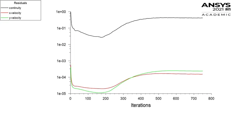
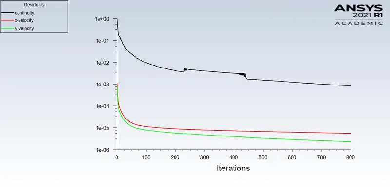
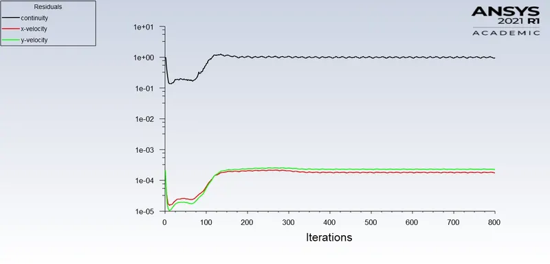
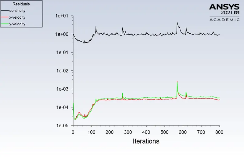
3. In both approaches, show that the flow has converged. That is, what quantities or plots need to be looked at to determine that the flow has converged?

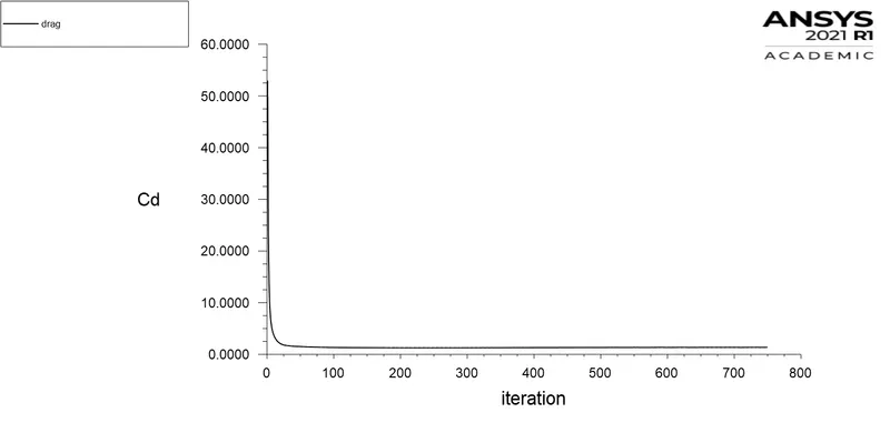
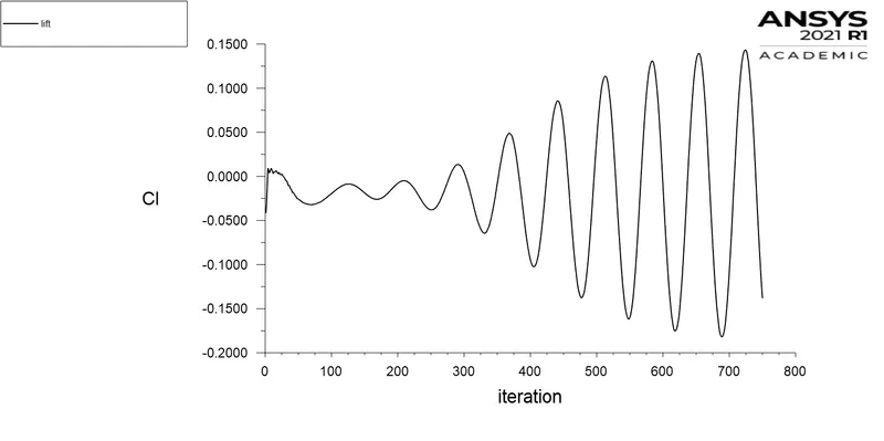
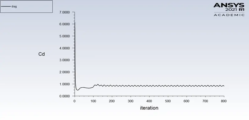
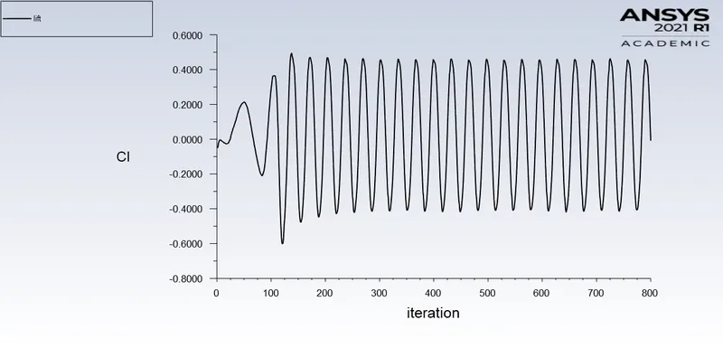
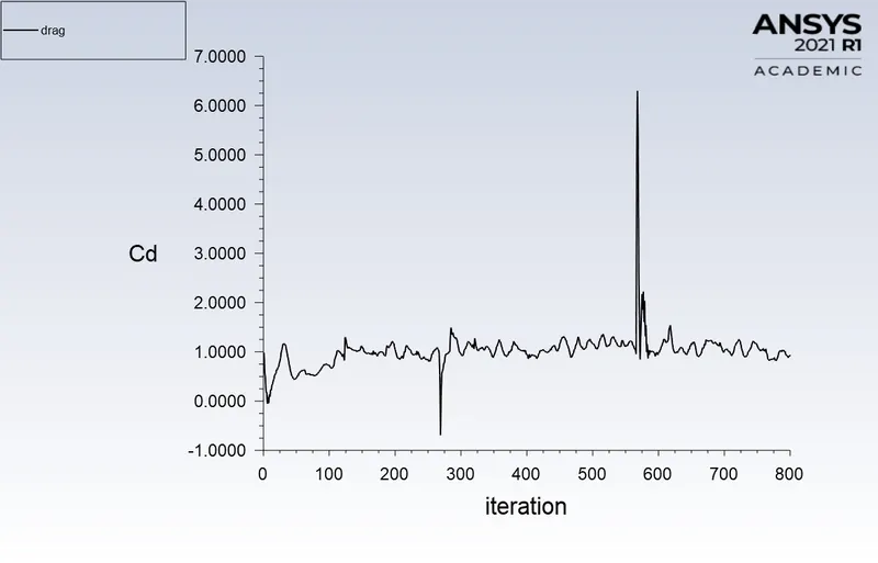
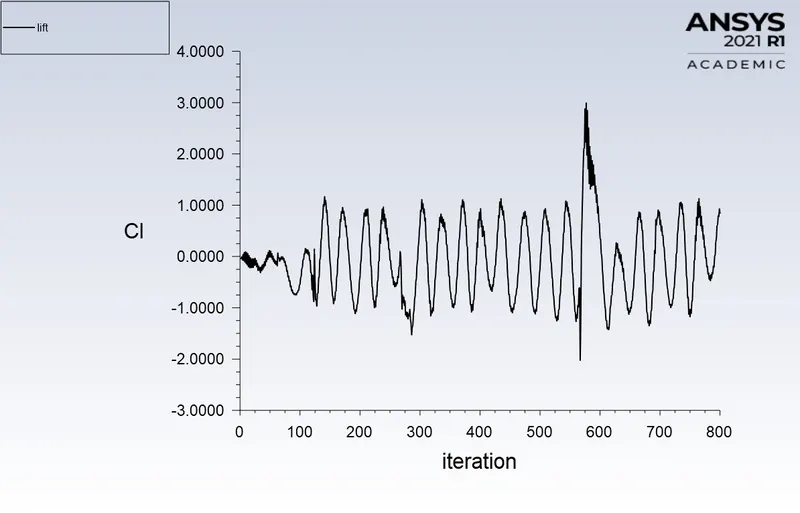
4. Plots of the coefficient of drag and lift.

5. Plots to show vortex shedding behind the cylinder.

6. Mention the preferred material at the end of the challenge submission page.

• THEORY:

1. Flow over cylinder:

In spite of extensive experimental and numerical studies of almost over a century, flow around a circular cylinder still remains a challenging problem in fluid mechanics, where intensive investigations are continued even today to understand the complex unsteady dynamics of the cylinder wake flow. Cross-flow normal to the axis of a stationary circular cylinder and the associated problems of heat and mass transport are encountered in a
wide variety of engineering applications. Both experimental measurements and numerical computations have confirmed the onset of instability of the wake flow behind a cylinder beyond a critical Reynolds number, leading finally to a kind of periodic flow identified by definite frequencies, well-known in the literature as the Von Karman vortex street. In case of laminar flow past cylinders with regular polygonal cross-sections, the flow
usually separates at one or more sharp corners of the cross-section geometry itself, forming a system of vortices in the wake on either side of the mid-symmetry plane. On the other hand, for a circular cylinder, where the point of flow separation is decided by the nature of the upstream boundary layer, the physics of the flow is much more complex than what its relatively simple shape might suggest.

2. Strouhal number:

In dimensional analysis, the Strouhal number is a dimensionless number describing oscillating flow mechanisms.

For large Strouhal numbers (order of 1), viscosity dominates fluid flow, resulting in a collective oscillating movement of the fluid "plug". For low Strouhal numbers (order of 10⁻⁴ and below), the high-speed, quasi-steady-state portion of the movement dominates the oscillation. Oscillation at intermediate Strouhal numbers is characterized by the buildup and rapidly subsequent shedding of vortices.

The Strouhal number is often given as

St=fDU′St=fDU′

Where,

f= frequency of vortex shedding

D= characteristic diameter of the cylinder

U'= fluid flow velocity

3. Co-efficient of drag:

In fluid dynamics, the drag coefficient(Cd)(Cd) is a dimensionless quantity that is used to quantify the drag or resistance of an object in a fluid environment, such as air or water. It is used in the drag equation in which a lower drag coefficient indicates the object will have a less aerodynamic or hydrodynamic drag. The drag coefficient is always associated with a particular surface area.

The drag coefficient of any object comprises the effects of the two basic contributors to fluid dynamic drag: skin friction and form drag. The drag coefficient of a lifting airfoil or hydrofoil also includes the effects of lift-induced drag. The drag coefficient of a complete structure such as an aircraft also includes the effects of interference drag.

The drag coefficient CdCd is defined as

Cd=2⋅Fdρu2ACd=2⋅Fdρu2A

where:

Fd is the drag force, which is by definition the force component in the direction of the flow velocity,

ρ i is the mass density of the fluid,

u and the flow speed of the object relative to the fluid is the reference area.

4. Co-efficient of lift:

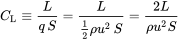
The lift coefficient (CLCL) is a dimensionless coefficient that relates the lift generated by a lifting body to the fluid density around the body, the fluid velocity, and an associated reference area. A lifting body is a foil or a complete foil-bearing body such as a fixed-wing aircraft. C_L is a function of the angle of the body to the flow, its Reynolds number, and its Mach number. The section lift coefficient c_l refers to the dynamic lift characteristics of a two-dimensional foil section, with the reference area replaced by the foil chord.

where

is the lift force,

is the relevant surface area and

q is the fluid dynamic pressure, in turn, linked to the fluid density, and to the flow speed.

A brief explanation to solve the flow over a cylinder

1. Geometry

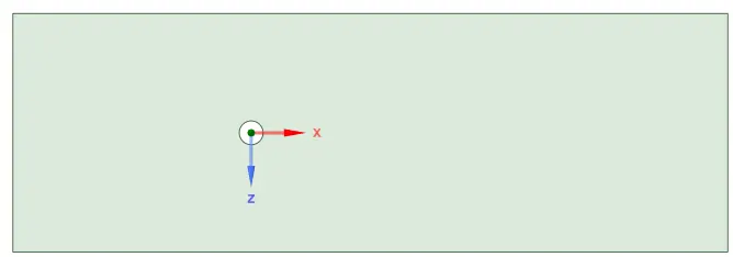
Creating the geometry by sketching using the line and circle command, circle diameter of 2m and the dimensions having 20X60m and the circle is placed 20m from the inlet.

2. Mesh

After the geometry is loaded we should mesh it and here I used 0.19m as the elemental size

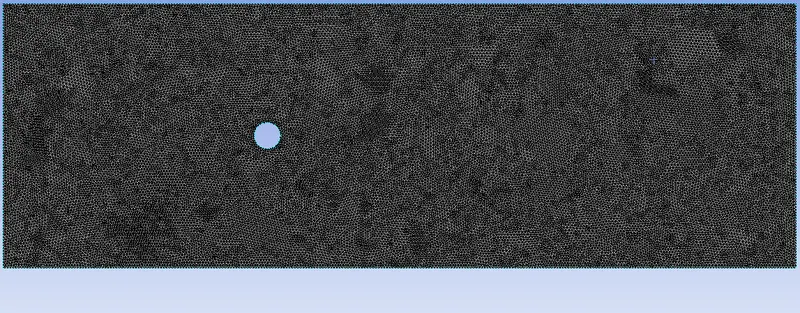
But in the meshing nodes, the shape is more quadrilateral than the triangle so we should do this by changing the method to the triangle in the insert option

After changing the node's shape into triangles we should improve the mesh around the cylinder by sizing in the mesh which is used to control precisely the mesh.

Then we should add inflation which is used to create the body-fitted mesh

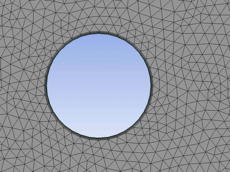
And we should name the boundaries as given below

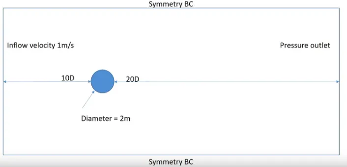
where the cylinder edge is named as the wall

3. Setting up Ansys fluent

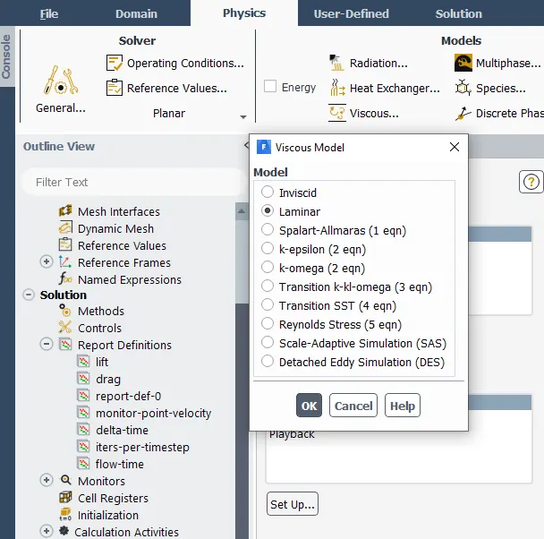
Before opening the set up we should update the mesh. Then we should change the viscous flow to laminar

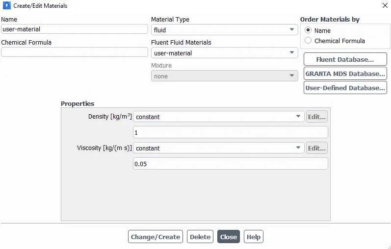
Open Materials and create a fluid that is to be used for the simulation for this case, it is air and also inputs the density and kinematic viscosity values.

Open Zones and input the inlet velocity as per the reynolds number and check if the fluid is updated.

Update the reference values which are located inside the setup on the right-hand side.

Fluent details/procedure:

a. laminar model

b. fluid: Air

c. Method of discretization: Simple

d. Density/kinematic viscosity: 1/0.05

e. Creating a monitor point behind the cylinder by selecting a point under surfaces in the results bar.

f. After creating the monitor point, create reports/plots for drag, lift, velocity wrt cylinder.

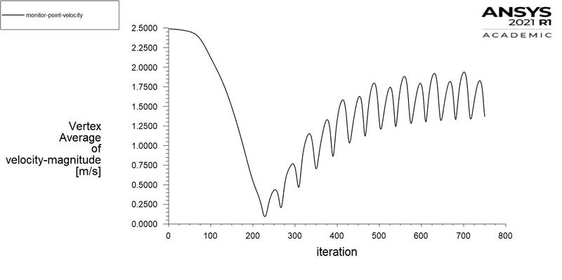
g. Create plots for the velocity at the monitor point to analyze the vortex shedding.

h. Use hybrid initialization for steady-state and standard for transient-state simulations.

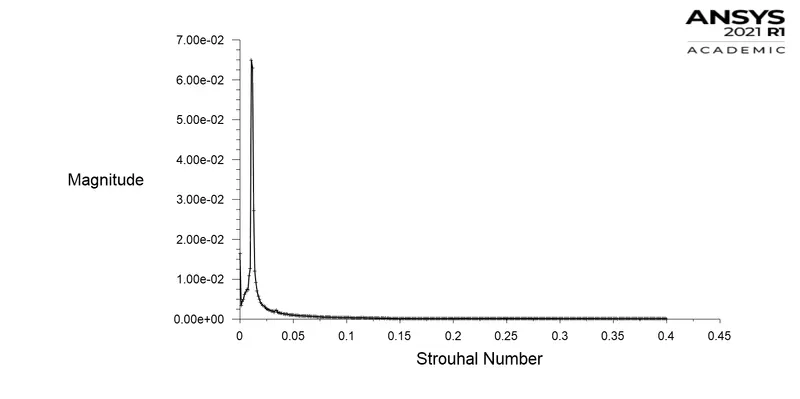
(i) Simulate the flow with the steady case and calculate the Strouhal number for Re=100 and velocity 2.5m/s.

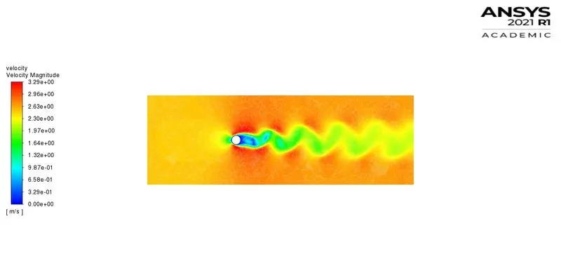
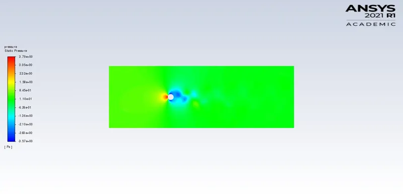
• Velocity and pressure contours

• Residuals plot

• Drag and lift coefficient

• velocity at the monitor point

• Strouhal number plot

(ii) Simulate the flow with the unsteady case and calculate the Strouhal number for Re=100 and velocity 2.5m/s.

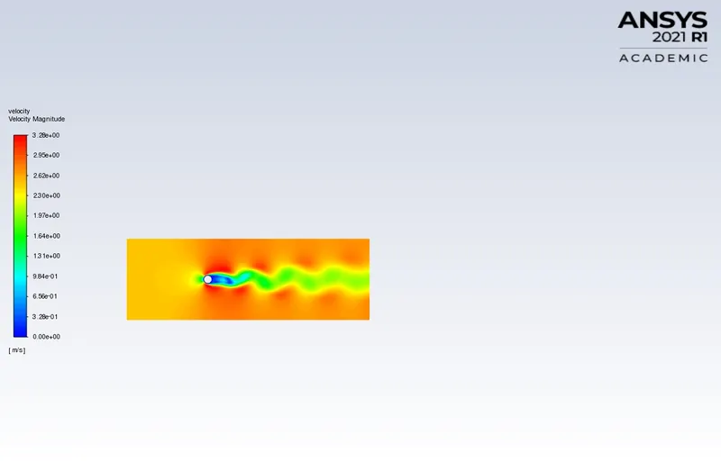
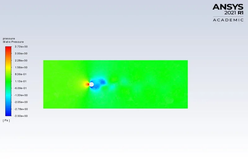
• Velocity and pressure contours

• Residuals plot

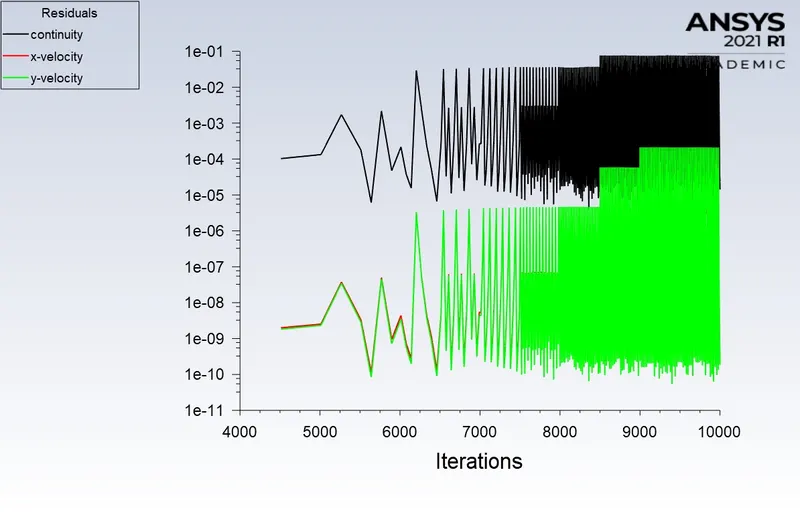
• Drag and lift coefficient

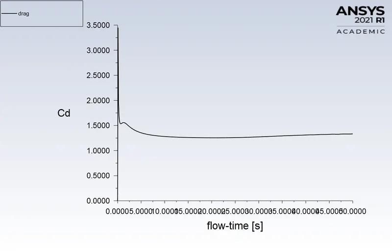
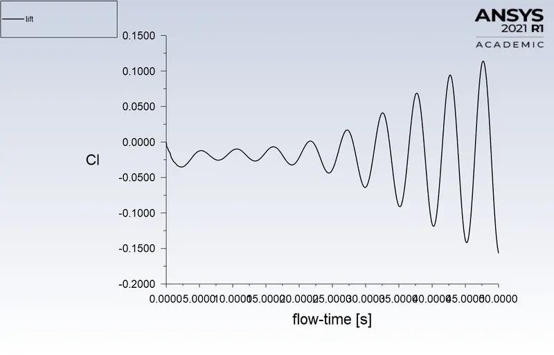
• velocity at the monitor point

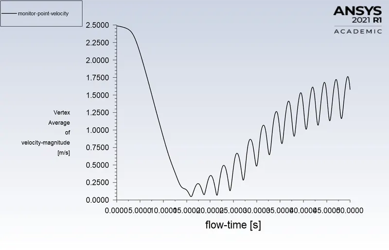
• Strouhal number plot

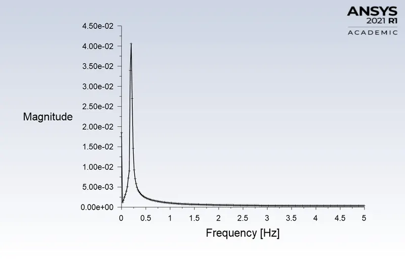
solver	CdCd	CLCL	Strouhal number
steady-state	1.365	-0.13	0.01333
unsteady-state	1.3336	-1.179	0.1996

Part-2

(i) Simulate the flow with the steady-state solver for Re=10.

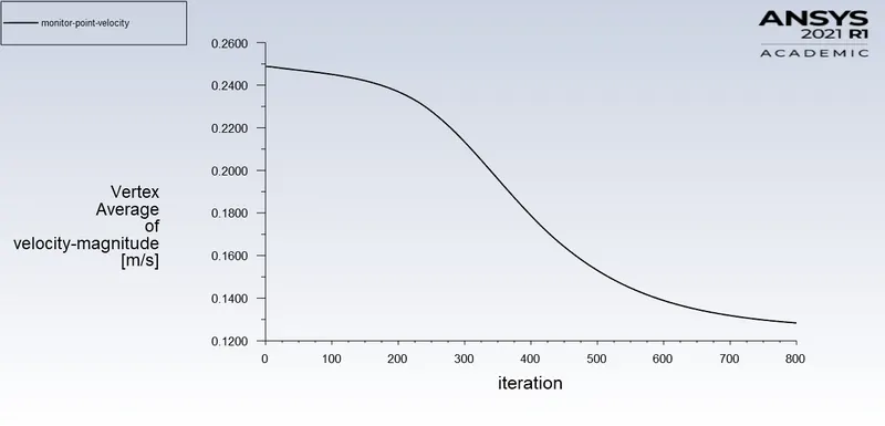
For Re=10 velocity v=0.25m/s

• Velocity and pressure contours

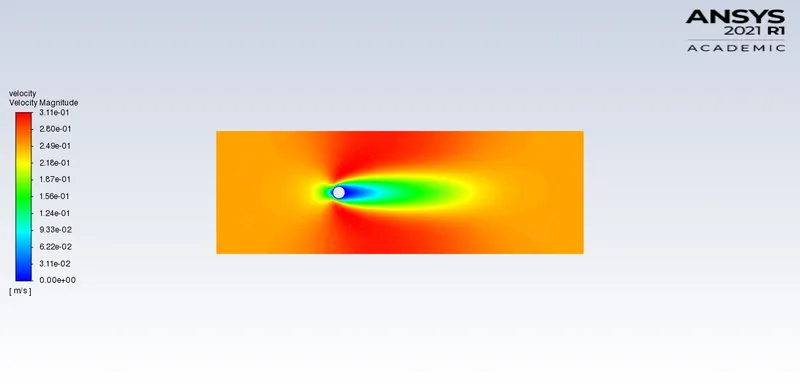
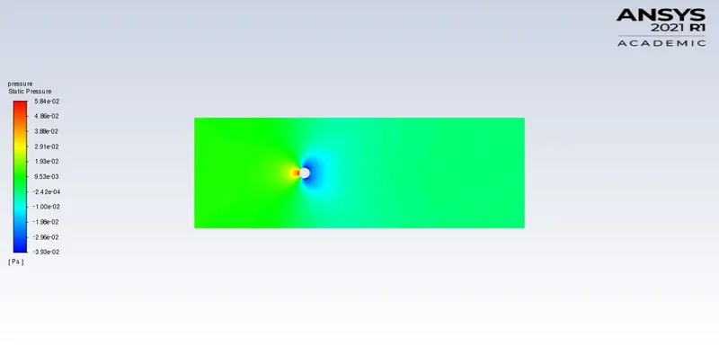
• Residuals plot

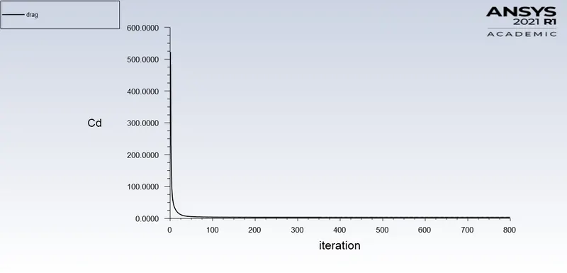
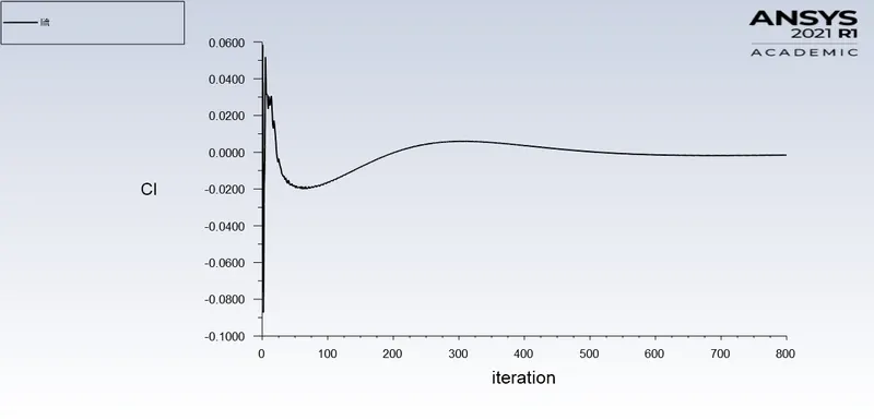
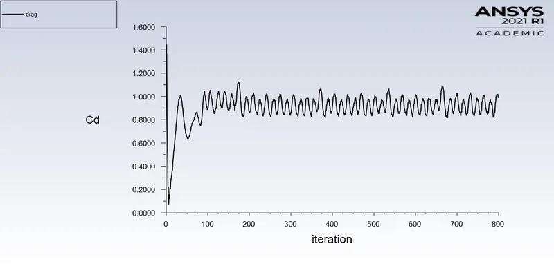
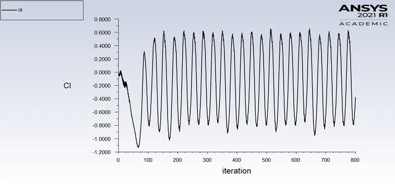
• Drag and lift coefficient

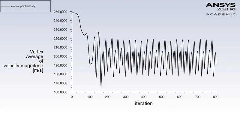
• velocity at the monitor point

(ii) Simulate the flow with the steady-state solver for Re=100.

For Re=100 velocity v=2.5m/s

• Velocity and pressure contours

• Residuals plot

• Drag and lift coefficient

• velocity at the monitor point

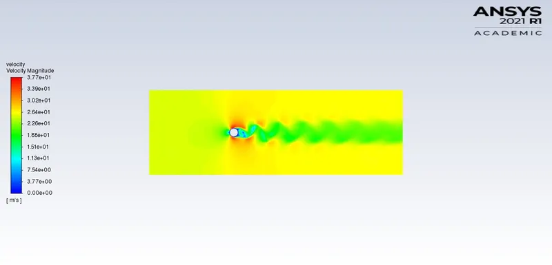
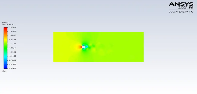
(iii) Simulate the flow with the steady-state solver for Re= 1000.

For Re=1000 velocity v=25m/s

• Velocity and pressure contours

• Residuals plot

• Drag and lift coefficient

• velocity at the monitor point

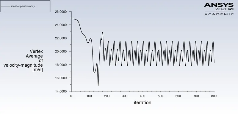
(iv) Simulate the flow with the steady-state solver for Re= 10000.

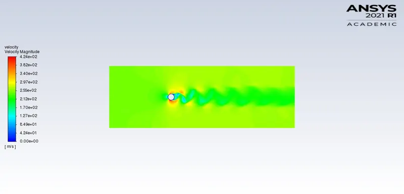
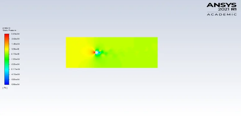
For Re=10000 velocity v=250m/s

• Velocity and pressure contours

• residual plot

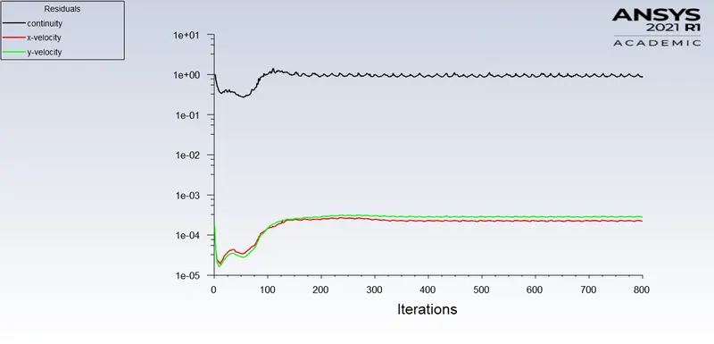
• Drag and lift Coefficient

• velocity at the monitor point

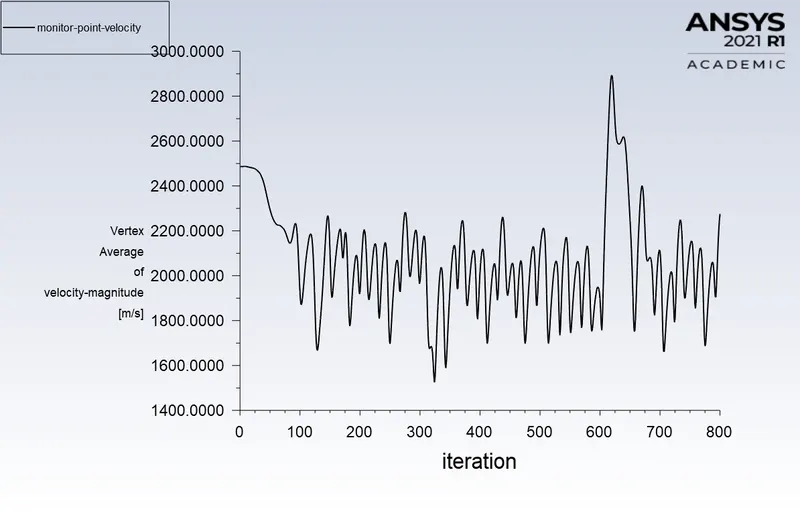
(v) Simulate the flow with the steady-state solver for Re= 100000.

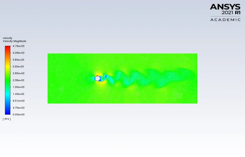
For Re=100000 velocity v=2500m/s

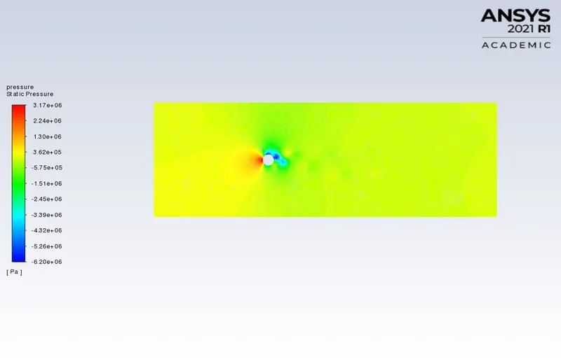
• Velocity and pressure contours

• residual plot

• Drag and lift Coefficient

• velocity at the monitor point

Result:

Drag and lift coefficient for different Re

Re	CdCd	CLCL
10	3.33	-0.00155
100	1.365	-0.13
1000	0.808	-0.00839
10000	0.9876	-0.373
100000	0.937	0.833

.Error wrt the theoretical values from the reference material,

Reynolds number	theoretical Cd	Numerical Cd	error
10	3.5	3.333	4.77%
100	1.4	1.365	2.5%

Conclusions:

• In the first case, the flow over a cylinder is simulated for both Steady and unsteady cases with Re=100, and with the results generated the phenomena of Von Karman Vortex Street are also observed.
• Necessary plots are plotted in order to observe that the flow is converged and the vortex shedding is happening.
• Contours are generated in order to observe the flow over a cylinder.
• By plotting Power Spectral Density vs Frequency, the Strouhal number is calculated.

• In the second case,
• six different simulations i.e (Re = 10,100,1000,10000,100000,1000000) are simulated to observe the behavior of the drag and lift coefficients by changing the Reynolds number.
• In order to observe the behavior of the drag coefficients for the simulations, the velocity of the flow is varied to change the Reynolds number and the rest of the parameters are kept constant.
• As we know if the Reynold number is less than 2000, then the flow in a pipe is Laminar. Hence we use the Viscous model = Laminar.
• For Re=10, it is observed that there is no formation of vortex shedding and in the rest of the cases, it is clearly observed.
• As per the basic conditions and parameters, the results are validated from the literature.
• As we refine the mesh we need to run more iterations.
• From the above table, it can be concluded that the error percentage is less than 5%.