Week 2 - Flow over a Cylinder.
AIM:
To simulate the flow over a cylinder and explain the phenomenon of Karman vortex street.
Objective:
PART-I
- Simulate the flow with the steady and unsteady case and calculate the Strouhal Number for Re= 100.
PART-II
- Calculate the coefficient of drag and lift over a cylinder by setting the Reynolds number to 10,100,1000,10000 & 100000. (Run with steady solver)
- Discuss the effect of Reynolds number on the coefficient of drag.
Karman vortex street:
A regular stream of vortices shed from a body placed in a fluid stream: investigated by Karman who advanced a formula for the frequency of the shed vortices in terms of the stream velocity and the dimensions of the body See also vortex street.
In fluid dynamics, a Karman vortex street is a repeating pattern of swirling vortices, caused by a process known as vortex shedding which is responsible for the unsteady separation of flow of a fluid around blunt bodies.
The flow around a (geometrically) two-dimensional circular cylinder is case that has been used both as a validation case and as a legitimate research case. At very low Reynolds numbers, the flow is steady and symmetrical. As the Reynolds number is increased, asymmetries and time-dependence develop, eventually resulting the famous Von Karmann vortex street, and then on to turbulence. The problem geometry is two-dimensional and there is some variation in the details (both geometry and boundary conditions) that can be used. A typical geometry is shown below (not to scale).
The exterior boundaries are generally placed very far from the cylinder surface to avoid interaction between the boundary conditions. Grid generation is not especially difficult, though care must be taken to properly resolve the near-wall region as the Reynolds number is increased.
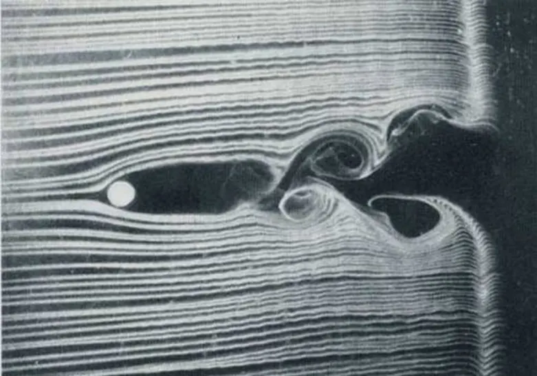
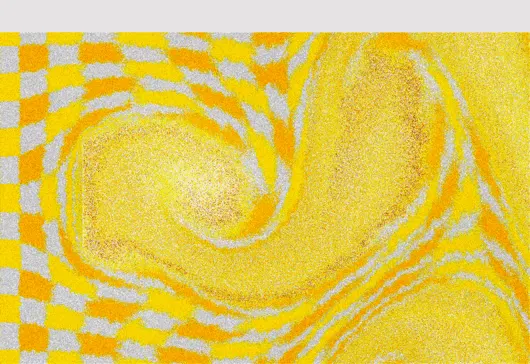 `
`
A vortex street will form only at a certain range of flow velocities, specified by a range of Reynolds numbers (Re), typically above a limiting Re value of about 90. The Reynolds number for a flow is a measure of the ratio of inertial to viscous forces in the flow of a fluid around a body or in a channel, and may be defined as a non-dimensional parameter of the global speed of the whole fluid flow, Reynolds number is given by
Re = ρVL / μ
Where,
ρ = density of the fluid.
V = free stream velocity
L = Length or hydraulic diameter
μ = dynamic viscosity
Vortex formation doesn’t occur at lower Reynolds number, when the Reynolds number increases the vortex formation starts proportionally with increasing Reynolds number. When the Reynolds number is sufficiently higher, Karman Vortex shedding occurs. This shedding can be symmetric at transition regimes and asymmetric at turbulent regimes. This vortex shedding oscillates periodically leading to a singing like occurrence, this is given mathematically by Strouhal number
St = fL / U
Where,
f = frequency of vortex shedding
L = characteristic length or the hydraulic diameter
U = flow velocity
Coefficient of Drag (Cd)= The coefficient of drag is a dimensionless quantity that is used to determine the drag or resistance of an object in a fluid environment such as air or water.
Formula:
Re = 2 Fd /ρ.a.v^2
ρ = kgm3
V = m/s
Cd = Coefficient of drag
Fd = Drag force
ρ = Density of the fluid
a = projected are of the object with respect to drag force calculated
V = Velocity of the fluid
The coefficient of lift (Cl) is dimensionless quantity that is used to determine the lift of an object in a fluid environment.
Formula:
Where
Cl = 2 ⋅ Fl / ρ ⋅ A ⋅ V 2
Cl = coefficient of lift
Fl = Lift force.
ρ = Density of the fluid
A= Projected area of the object w.r.t which drag force is calculated.
V= Velocity of fluid
As usual we have to follow five major steps for these simulations they are
- Geometry
- Meshing
- Set-up
- Solution
- Result
Step 1 is geometry spaceclaim:
First step is we have to open the Fluent, right click on the geometry and select New Space Claim Geometry. The space claim application opens, select FILE > NEW and we can create a geometry. Use SKETCH option and make a sketch as follows. First, we have to make a circle of 2m.
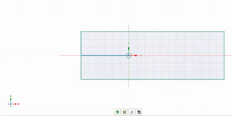
The diameter of circle is 2m, and the rectangular surface of 20m width and 60m length the geometry is shown below
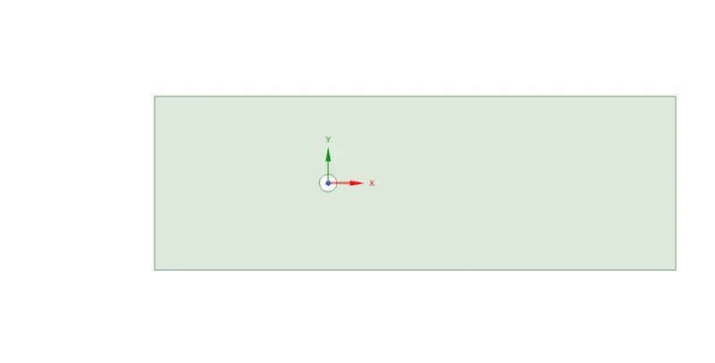
Once we created the geometry after we have to good to go meshing process.
Step 2 is Meshing process:
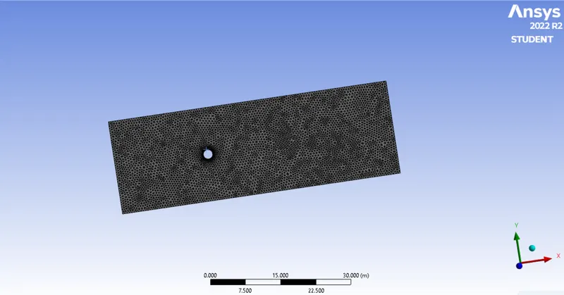
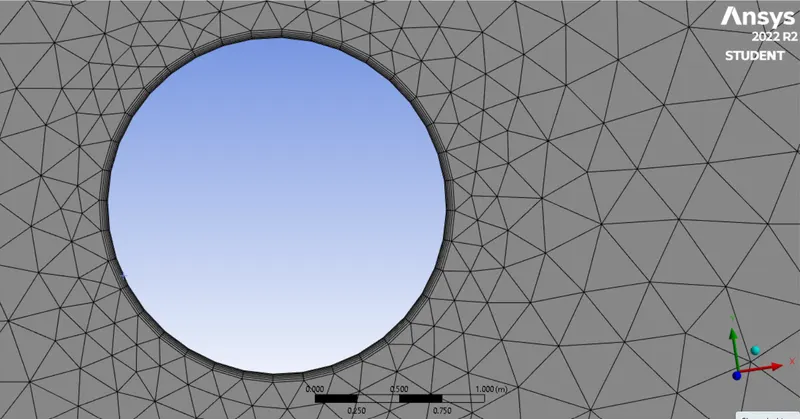
In the meshing process we Have to right clicking on the Mesh and selecting edit opens the Mesh window. In the Mesh window is automatically preloaded with the geometry and then clicking on the GENERATE MESH should create a mesh automatically. The default mesh is mixed mesh here, but we are interested in tria type mesh. So, right clicking on the mesh and going to INSERT > METHOD > ALL TRIANGLES. In this simulation we have to add inflation layers with 0.5 as first layer thickness and add 6 layers. The desired mesh size we can use is 500 mm. We have to create a monitoring point at 8m from the cylinder in the wake region. In this monitoring point used to study the average velocity. After completed the meshing process we should give named selection option it is used to create named surface such as Inlet, Outlet, Wall by selecting the respective faces and using the ‘N’ button and name them as symmetry. Once we complete the meshing process we should move next process.
Step 3 is ste-up:
Solver type: Pressure based
Velocity formulation: Absolute
Solver Time: Steady State
Viscous: laminar
Under the cell zone conditions, we have to select the volume and it should show type as fluid by default. After that we can able to proceed to define boundary conditions, as follows
Inlet X: velocity magnitude = 2.5 m/s (For Re 100)
Outlet should be a pressure outlet.
upper and lower walls can be set as symmetry.
Similarly, we have to make a report for lift coefficient, and for Vertex average velocity we can use Solution > Reports > Definitions > New > Vertex average > Velocity, and for drag we can use Solution > Reports > Definitions > New > Force > Drag, and for lift we can use Solution > Reports > Definitions > New > Force > lift.
We have to give input compute from INLET in reference values and in the initialization as well.
Now, it's time to start the simulation. In order to start the simulation for the above set up physics, we need to initialize the entire flow field by clicking on the t=0 initialize icon.
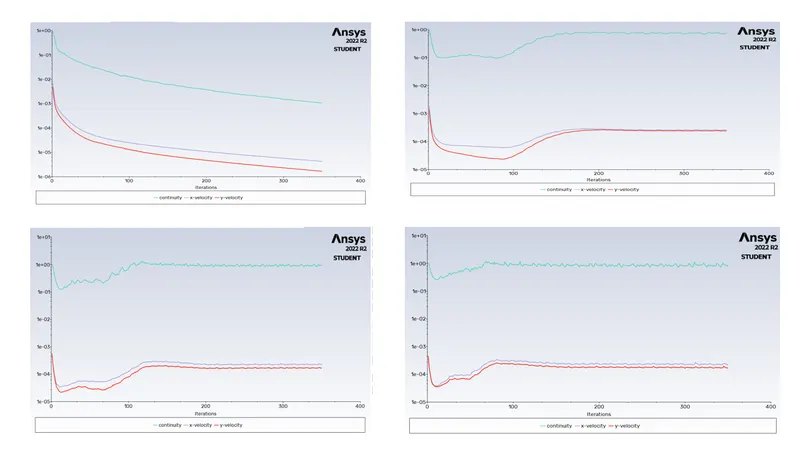
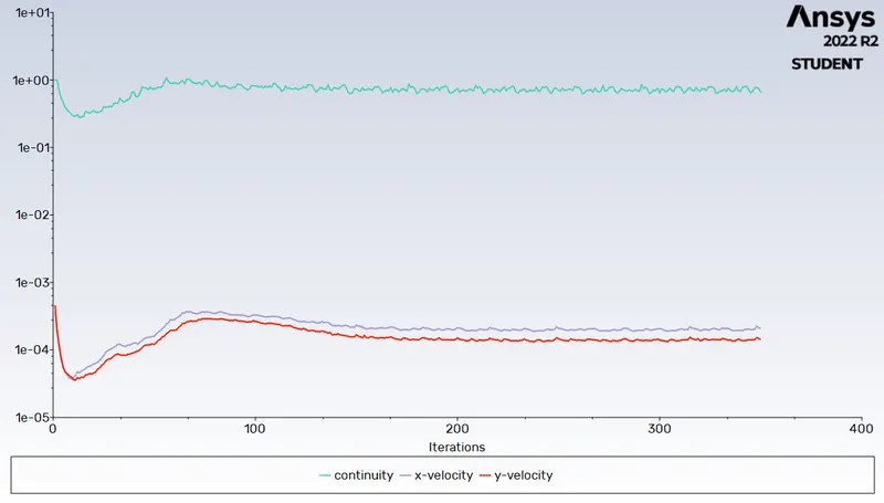
In the Run Calculation we can input the number of iterations to be run (in this case 350) and clicking on the Calculate should start the iterations.
After iterations, we get scaled residuals, average temperature plot and standard deviation plots
In Re = 100 we have to give both time states such us steady state and transient state.
RESULTS:
Final step of the simulation is Result option so we have to Right clicking on the Results should open the Post processor. Default it will show wireframe mood, we can turn on the symmetry 1 to view contours and vectors.
We have to Selecting the Vector and selecting the symmetry 1 plane creates a velocity vector.
Similarly in the setup and solution, all contours and plots can be created here,
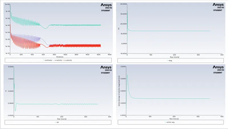
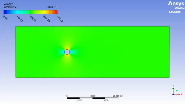
In this simulation we have to create an animation of the velocity contour by using AUTOSAVE option during the solution and clicking on ANIMATE select make movie and save it. In Case 2 (Re 100, Transient), we can simply Duplicate the existing Case 1 Fluent file. Change the type to TRANSIENT in the Setup and add time step size as 0.01 and no. of time step as 1000 and run the simulation and collect the data.
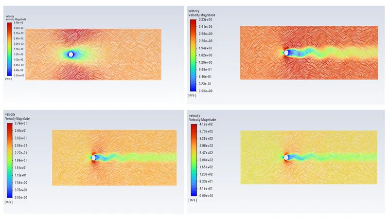
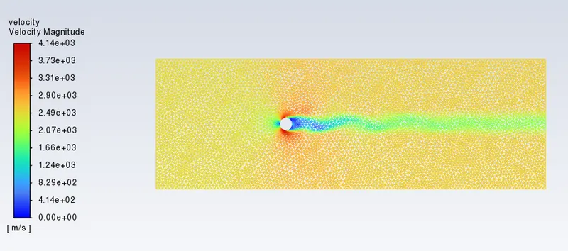
Similarly, we can follow the above procedure for the other cases from Re 10 to Re 100000, using steady flow in fluent solver. with velocities as 0.25 m/s for Re 10 upto 2500 m/s for Re 100000, with multiplication factor of 10 for each Reynolds number respectively.
Re 10 to 10000 Residual plots:
Re 100000 Residual plot:
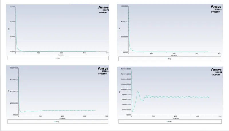
Re 10 to 10000 drag plot:
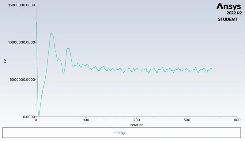
Re 100000 drag plot:
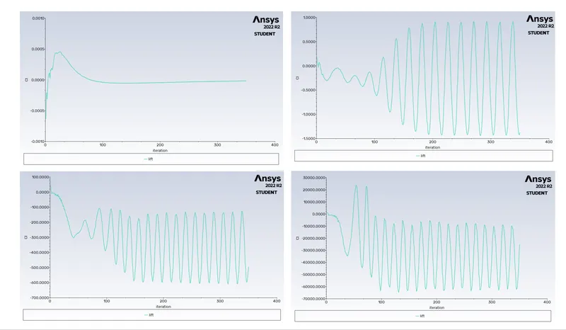
Re 10 to 10000 lift plots:
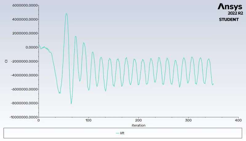
Re 100000 lift plot:
Re 10 to 10000 vertex plots:
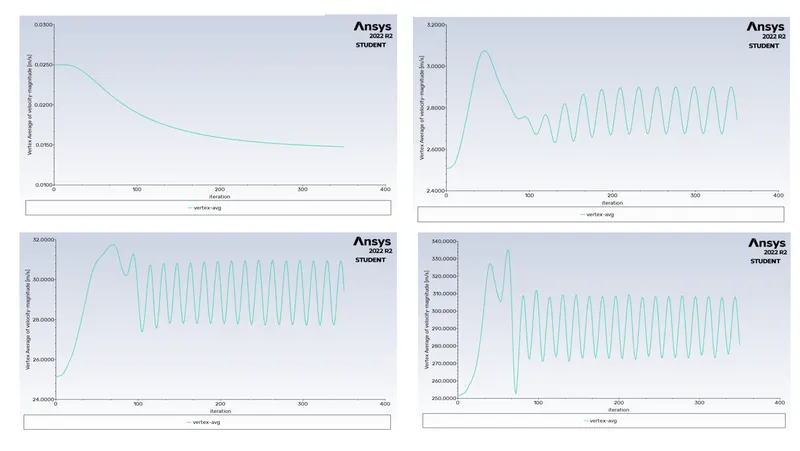
Re 100000 vertex plot:
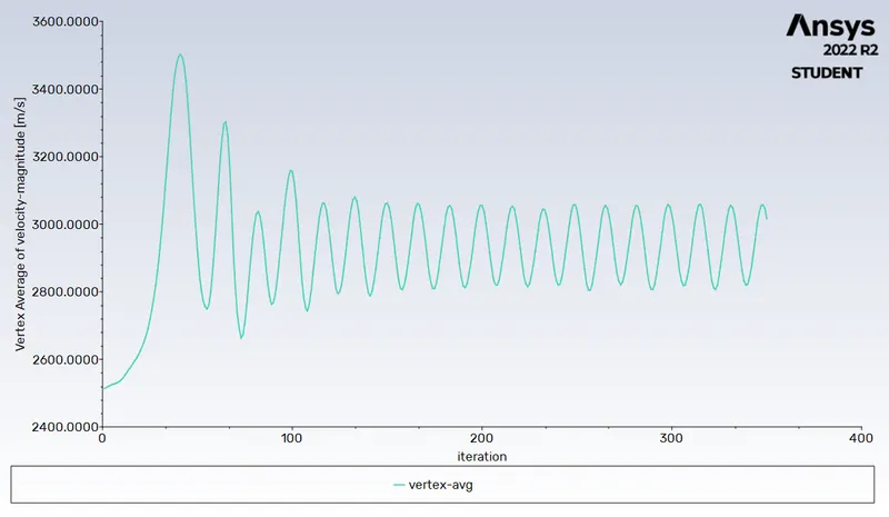
Re 10 to 10000 pressure plots:
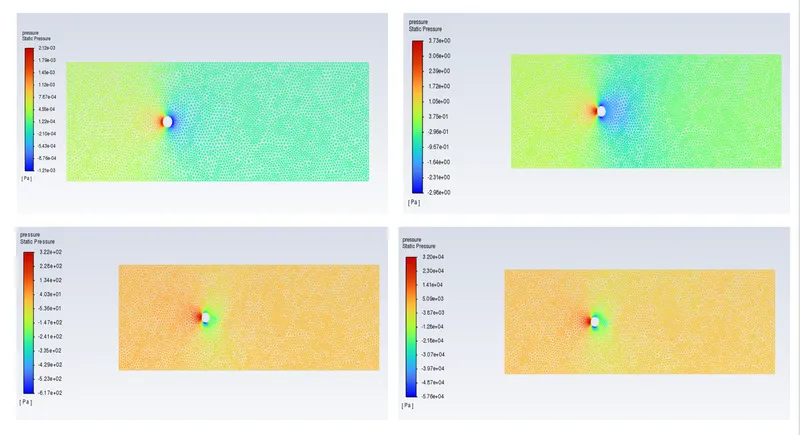
Re 100000 pressure plot:
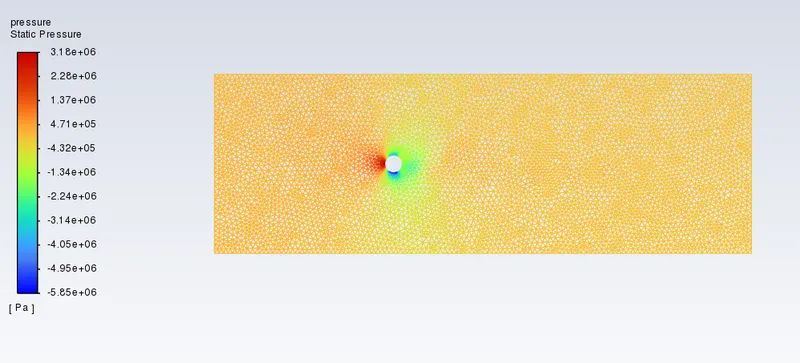
Re 10 to 10000 velocity plots:
Re 100000 velocity plot:
Re 100 transient plots:
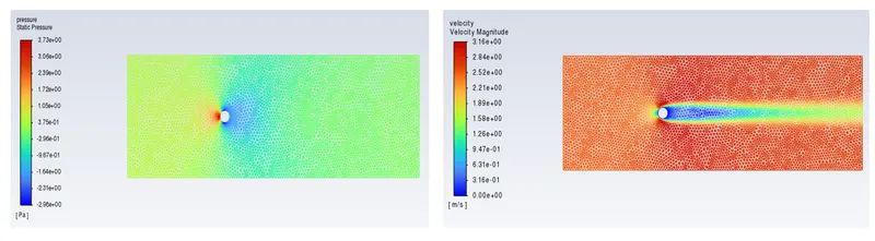
Re 100 transient velocity and pressure plot:
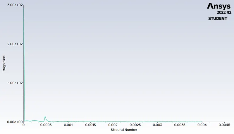
Strouhal numbr vs magnitude plot:
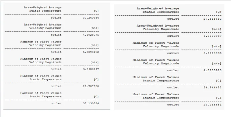
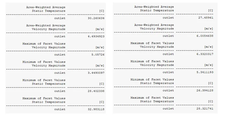
Re 10 to 10000 values image:
Animation GIF :
Inference:
The challenge has been divided into two parts first part is steady& second part is unsteady state simulations have been performed for Re 100 & Strouhal number has been calculated using analytical method & later compared with the fluent result.
In the second part of the simulation has been carried out for various Re numbers in steady state condition. Vortex shedding & Karman vortex street was unable to visualize for Re 10 because these two phenomena doesn’t occur below Re 40. The drag coefficient & lift coefficient has been comparing for all simulations.
The result values of the lift, drag, and vertex average:
Re Cd Cl Vertex Average Velocity(m/s)
10 3.431 -0.0026 0.240
100 1.335 -0.054 11.784
1000 0.726 -0.085 14.738
10000 1.615 -0.048 12.556
100000 0.869 -0.0491 15.459
Conclusion:
Finally, the conclusion of the challenge we had to completed the simulation of flow over a cylinder has been carried out to study the vortex shedding phenomena & visualizing von Karman vortex street.
The challenge has been divided into two parts first part is steady& second part is unsteady state simulations have been performed for Re 100 & Strouhal number has been calculated using analytical method & later compared with the fluent result.
In the second part of the simulation has been carried out for various Re numbers in steady state condition. The drag coefficient & lift coefficient has been comparing for all simulations.
Reference:
https://www.sciencedirect.com/science/article/pii/S0307904X08000243