Week 2 - Flow over a Cylinder.

Flow over a Cylinder

AIM:-

Simulate the flow over a cylinder and explain the phenomenon of Karman vortex street.

OBJECTIVE:-

Part-I

1. Simulate the flow with the steady and unsteady case and calculate the Strouhal Number for Re= 100.

Part-II

1. Calculate the drag and lift coefficient over a cylinder by setting the Reynolds number to 10,100,1000,10000 & 100000. (Run with the steady solver)
2. Discuss the effect of the Reynolds number on the coefficient of drag. [ Results should be validated with any standard literature and error should be within 5 %]

THEORY:-

• Flow over a cylinder is important in many industrial applications like the cooling of iron or cylindrical pipes. Circular pipes have more application in heat exchangers. High-temperature flue gases flow over a circular cylinder in a cross flow. Depending on the flow rate, fluid properties, and size of the cylinder, the flow can be laminar, transition, or turbulent.
• Flow past a cylinder is a common problem in fluid mechanics, highlighting the Von-Karman vortex shedding effect.
• A von Kármán vortex street (named after the fluid dynamicist Theodore von Kármán) is a phenomenon in fluid dynamics occurring with turbulent flow at a high Reynolds number. It consists typically of a pattern of swirling vortices in alternating directions that are caused, for example, by the unsteady separation of a fluid flowing over a rapidly moving cylinder. An empirical relation proposed by Strouhal gives , where is the vortex shedding frequency, is the diameter of the cylinder and is the flow velocity. For a fluid with kinematic viscosity , the Reynolds number is generally in the range of 100 to 10^7 to exhibit this behavior. The vortex shedding frequency describes the rate at which vortices are formed in the wake of the moving cylinder. This phenomenon can sometimes cause vibrations near the frequency in wires or antennas subjected to high winds.

Reynolds number

The term Reynolds number is the ratio of inertia force to the viscous force present in the fluid.
It is denoted by the symbol Re.

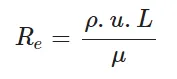
Where,
ρ = Density of fluid
u = Average velocity of the fluid
L = Characteristic length
μ = Dynamic viscosity of the fluid

Strouhal number

The Strouhal number represents the ratio of inertial forces due to the local acceleration of the flow to the inertial forces due to the convective acceleration. Depending on the time scale of the problem, this ratio may be of order unity, and therefore its importance is not obvious.

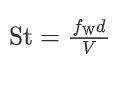
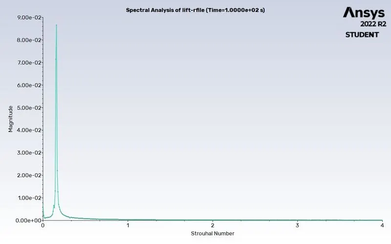
f_W being the vortex shedding frequency, V the approach flow velocity, and d the projected width normal to the flow direction.

It is used to describe oscillating flow mechanisms.

Coefficient of Drag

• The drag coefficient is a dimensionless quantity that is used to quantify the drag or resistance of an object in a fluid environment, such as air or water.
• The drag coefficient is a function of several parameters like the shape of the body, Reynolds Number for the flow, Froude number, Mach Number, and Roughness of the Surface.

Coefficient of Lift

• The lift coefficient (C_L) is a dimensionless coefficient that relates the lift generated by a lifting body to the fluid density around the body, the fluid velocity, and an associated reference area.
• C_L is a function of the angle of the body to the flow, its Reynolds number, and its Mach number.

PART I

We need to simulate the flow with the steady and unsteady case and calculate the Strouhal Number for Re= 100.

Modeling approach

• In this challenge, the flow is assumed to be two-dimensional and incompressible. The effects of body forces and viscous dissipation are neglected in this study.
• The thermophysical properties of the dummy fluid are assumed to be constant.
• Only laminar flow is considered in this case.

Geometry

• Open Spaceclaim.
• Use the Circle tool and create a circle at the origin with a diameter of 2m.
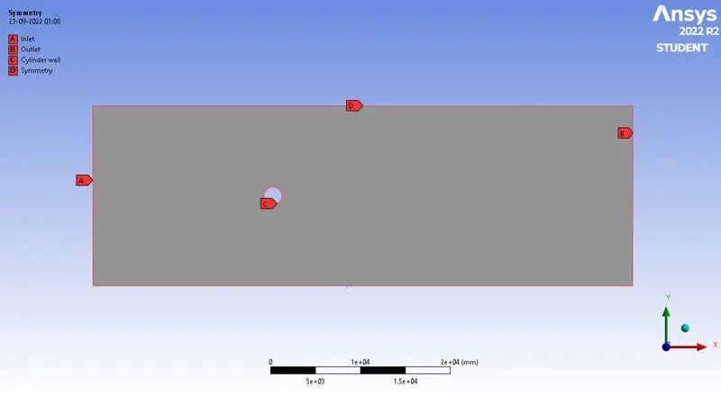
• Use the Line tool to create an outline according to the given dimensions.
• After that use the Rectangle tool and create a rectangle with sides of 20m and 100m.

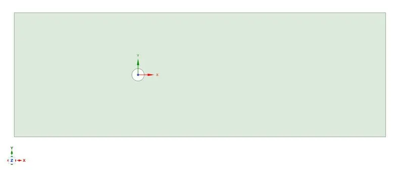
• Now use the Pull command to convert this 1D geometry into 2d geometry. After clicking on the Pull command, select the geometry.
• After that delete the construction lines and inner circle if present.

Mesh

• Open the Mesh window and use 'Generate mesh' to mesh the geometry.
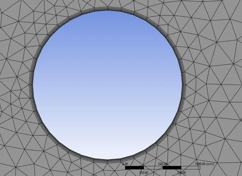
• To obtain only triangular mesh elements, go to mesh > insert > methods > select triangular mesh type. Here the element size is taken as 500mm.

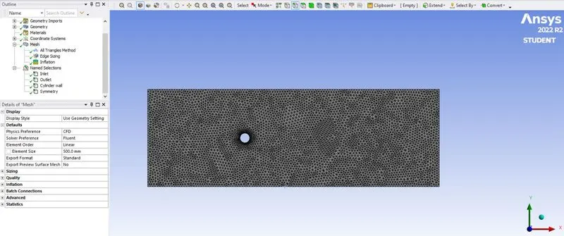
• To obtain a smooth surface around the circular geometry, we can use the Sizing option. For that go to mesh > insert > sizing. Select 36 divisions in this case.
• Now we can add inflation layers around the circle. For that go to mesh > insert > inflation. Select the number of layers and the thickness of the first layer.

• Name the boundaries as inlet, outlet, Cylinder wall, and symmetry.

• We are using the same geometry and mesh for both steady and transient conditions.

Setup for Steady case

REYNOLDS NUMBER 100

1.	Solver	Steady State
2.	Energy Equation	Off
3.	Model	Laminar
4.	Inlet	Velocity Inlet (2.5m/s)
5.	Outlet	Pressure outlet
6.	Material (Fluid)	User-defined (viscosity is 0.05 Kg/(m-s) and density = 1kg/m3)

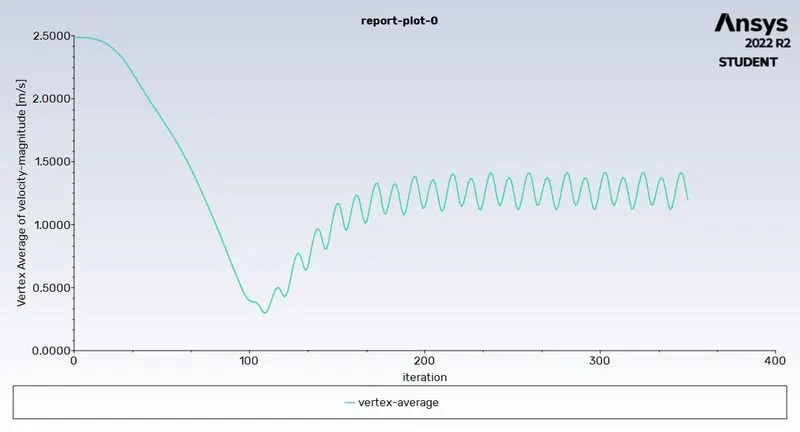
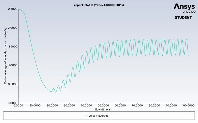
• Create a monitor point behind the cylinder by selecting the Point under surfaces in the Results bar. The point should be at a distance of at least 4 times the diameter of the cylinder.

• After creating the monitor point, create reports for Drag, Lift, and Vertex average velocity.

• Create contours for the velocity at the monitor point to analyze the vortex shedding.

• Select the solution method as 'SIMPLE' (pressure-velocity coupling).

• Run the simulation for 350 iterations after performing the Hybrid initialization.

Setup for Transient case

• The setup, in this case, is similar to the steady one.
• Here we select the Transient solver in place of the steady state solver.
• In place of iterations, here we have time steps and the number of time steps. We take the time step as 0.1s and the number of time steps as 1000 which gives us a time of 100s.

Results

Case 1 (Steady state)

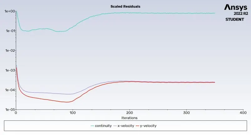
• Residual Plot

• Vertex average velocity at the monitor point

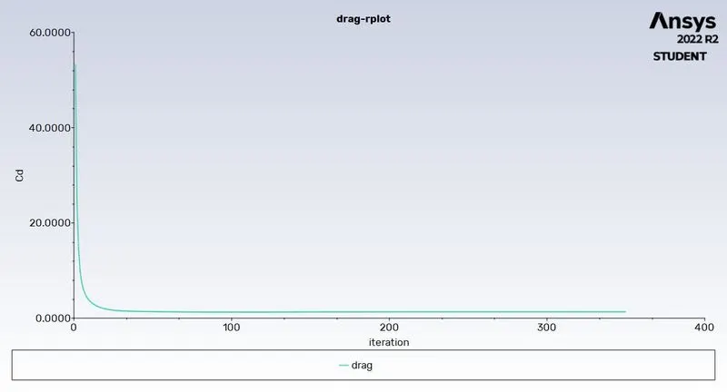
• Drag coefficient

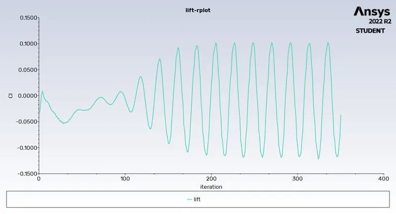
• Lift coefficient

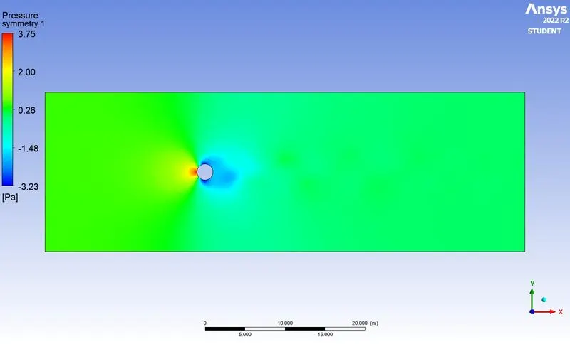
• Pressure contour

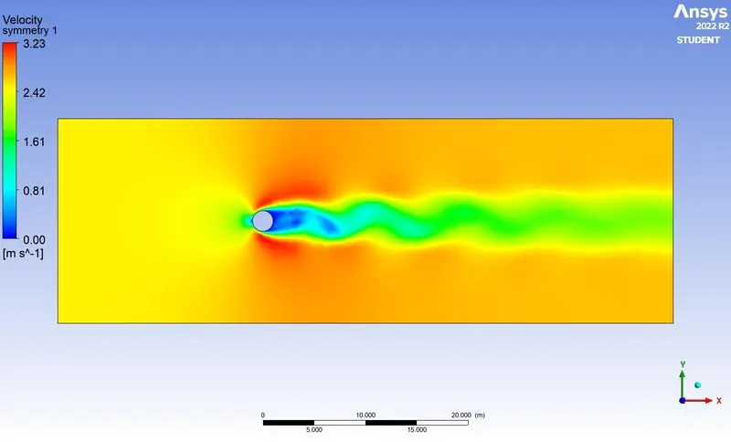
• Velocity contour

• Strouhal number

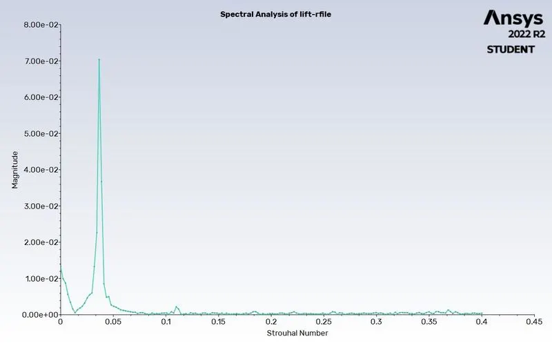
Case 2 (Transient state)

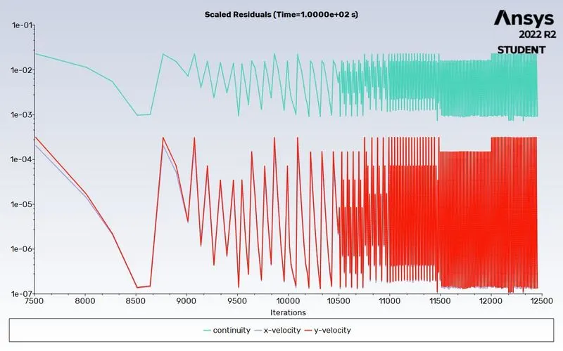
• Residual Plot

• Vertex average velocity at the monitor point

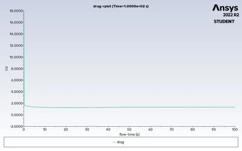
• Drag coefficient

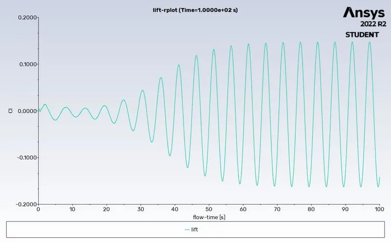
• Lift coefficient

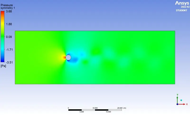
• Pressure contour

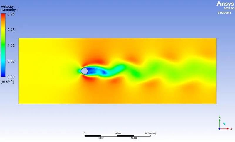
• Velocity contour

• Strouhal number

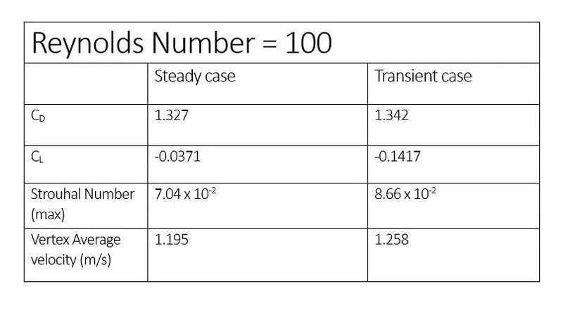
Comparison Table

PART II

• Here we need to calculate the drag and lift coefficient over a cylinder by setting the Reynolds number to 10,100,1000,10000 & 100000. (Run with the steady solver)
• The geometry and mesh used will be similar to Part I of this challenge.
• In the Setup, all the entered inputs remain the same except the inlet velocity of the fluid. For Reynolds number of 10, the inlet velocity is set as 0.25 m/s.
• Subsequently, for a change in Reynolds number by a factor of 10, we need to multiply the inlet velocity by 10.
• We will create reports for drag, lift, and vertex average velocity.

RESULTS

Case 1 (Re = 10)

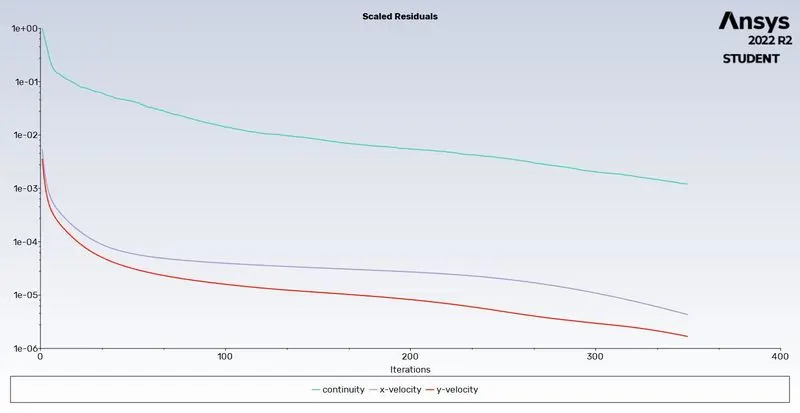
• Residuals plot

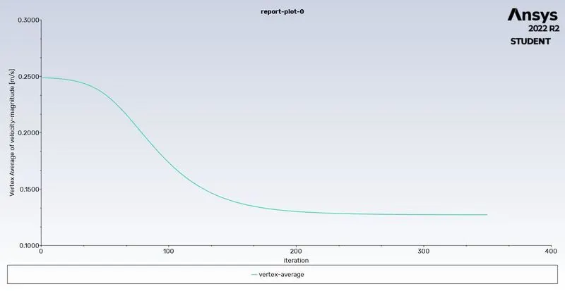
• Vertex average velocity at the monitor point

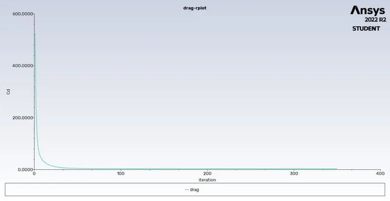
• Drag coefficient

• Lift coefficient

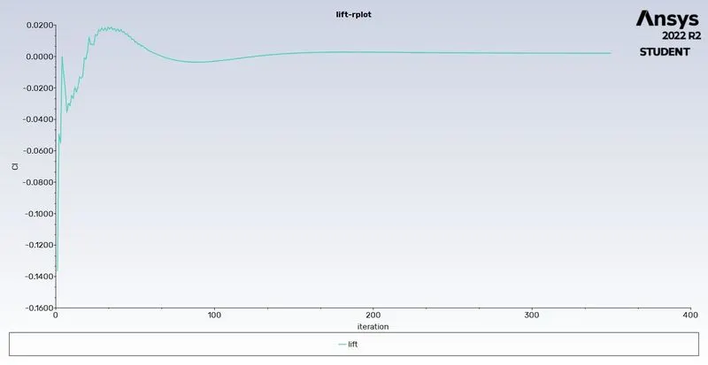
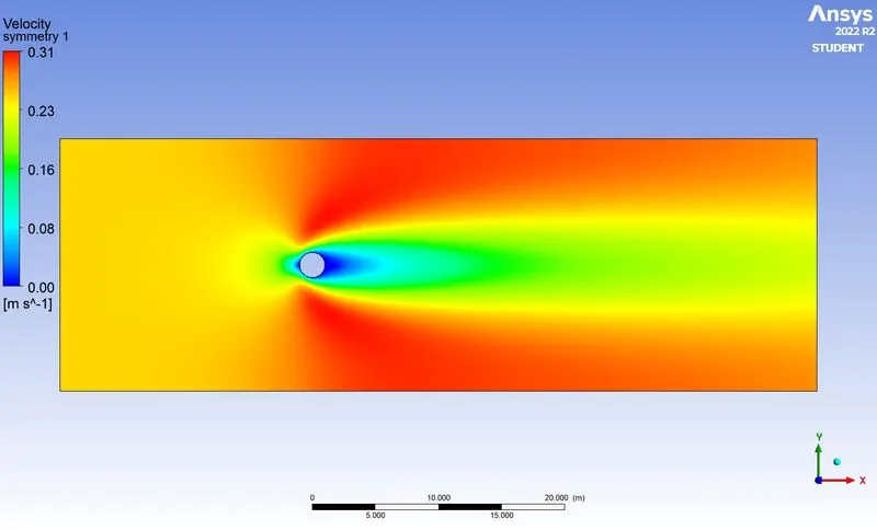
• Velocity contour

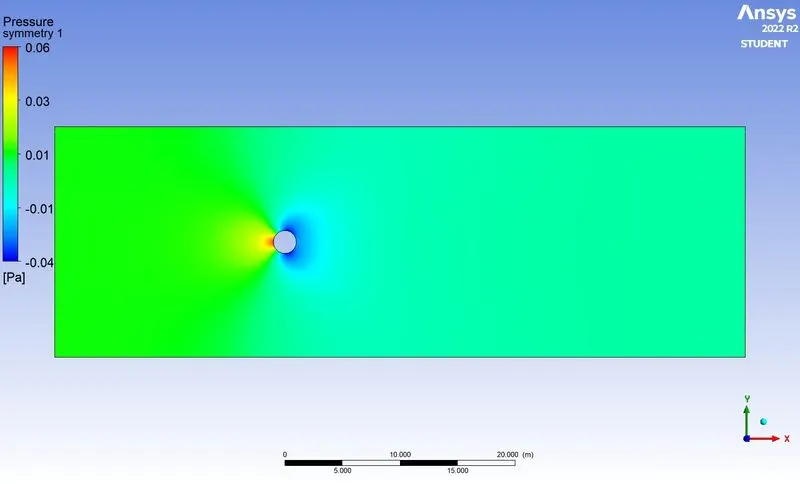
• Pressure contour

Case 2 (Re = 1000)

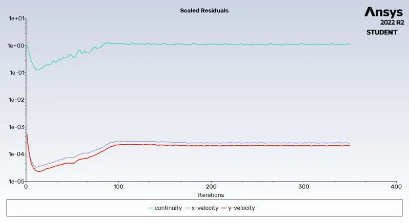
• Residuals plot

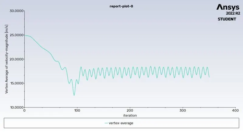
• Vertex average velocity at the monitor point

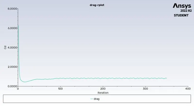
• Drag coefficient

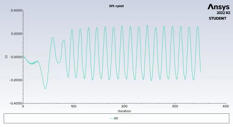
• Lift coefficient

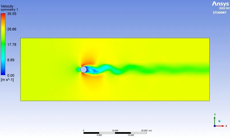
• Velocity contour

• Pressure contour

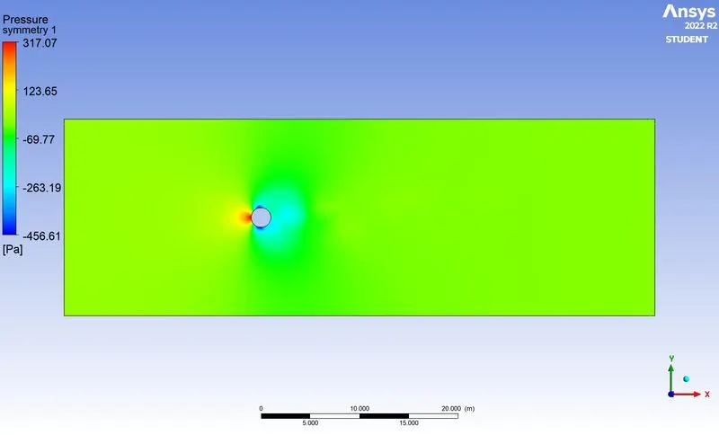
Case 3 (Re = 10000)

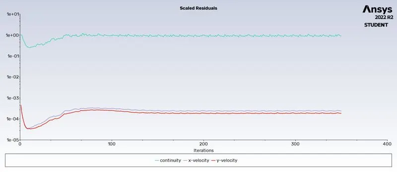
• Residuals plot

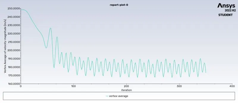
• Vertex average velocity at the monitor point

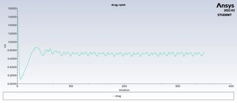
• Drag coefficient

• Lift coefficient

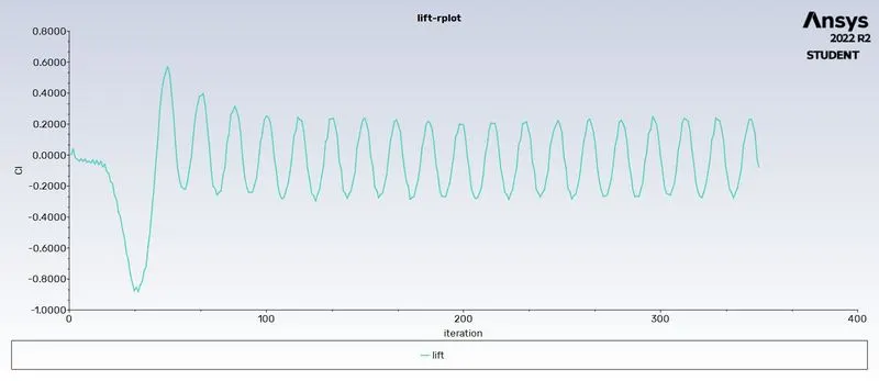
• Pressure contour

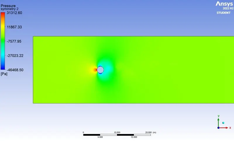
• Velocity contour

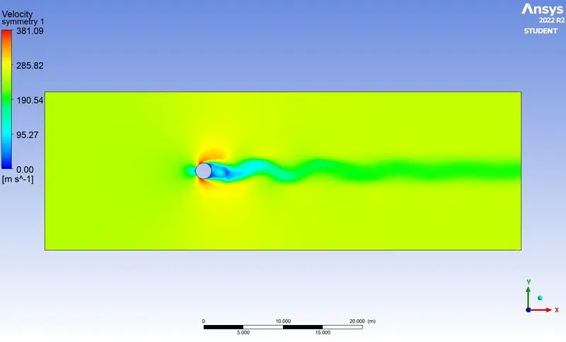
Case 4 (Re = 100000)

• Residuals plot

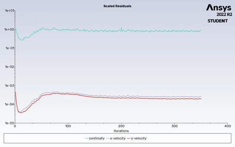
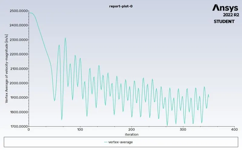
• Vertex average velocity at the monitor point

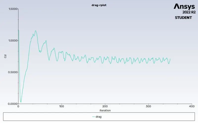
• Drag coefficient

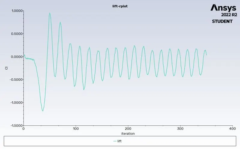
• Lift coefficient

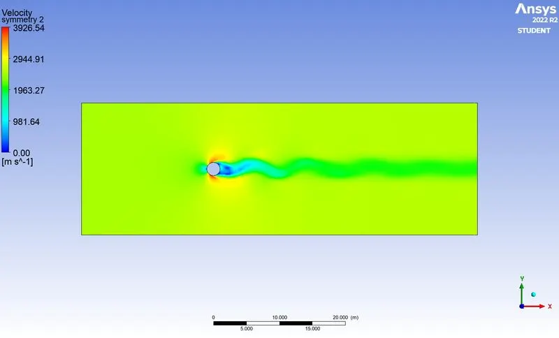
• Velocity contour

• Pressure contour

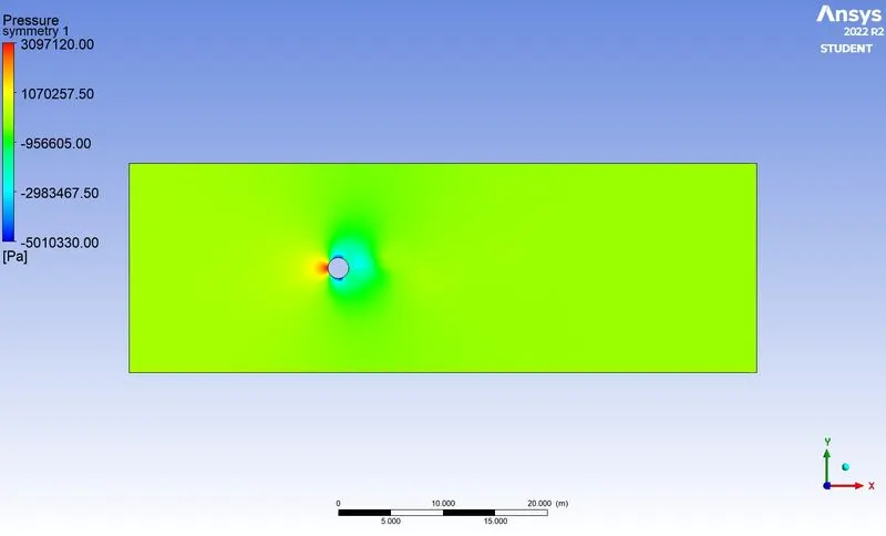
Case 5 (Re = 100)

• The results have been already mentioned in Part I and are the same for this case.

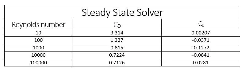
Comparison Table

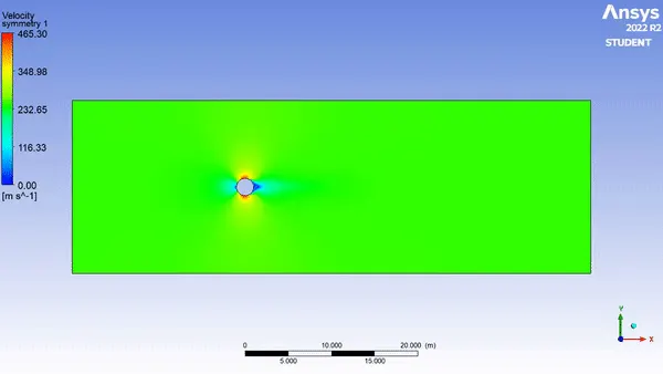
Animation for Re = 10000

CONCLUSIONS

1. From the above table, we can say that when the Reynolds number increases, the coefficient of drag decreases. This data is compared with the research paper. For Re=100, the research paper value for the coefficient of drag is 1.3353, and obtained value from the simulation is 1.327. Percentage of error=0.62% (less than 5%).
2. For Re=10, it is observed that there is no vortex shedding.
3. The von Karman vortex street can be observed when the Re number is greater than 100.
4. The wake region behind the cylinder increases with the increase in the value of the Reynolds number.

References:

1. https://thermopedia.com/content/1247/
2. https://www.sciencedirect.com/science/article/pii/S0307904X08000243 - Reference Journal
3. https://www.sciencedirect.com/topics/engineering/vortex-shedding
4. https://cfdflowengineering.com/cfd-modeling-of-flow-over-a-cylinder/
5. https://www.sciencedirect.com/topics/engineering/strouhal-number