Week 2 - Flow over a Cylinder.

Aim:

The Aim of the experiment to set up a flow analysis over a 2D cylinder using Ansys fluent and study the Karman Vortex Street phenomena using steady and Transient flow conditions.

OBJECTIVE:

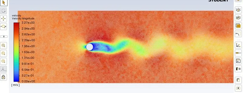
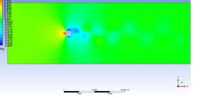
1. To simulate the flow with the steady and unsteady case and calculate the Strouhal Number for Re= 100
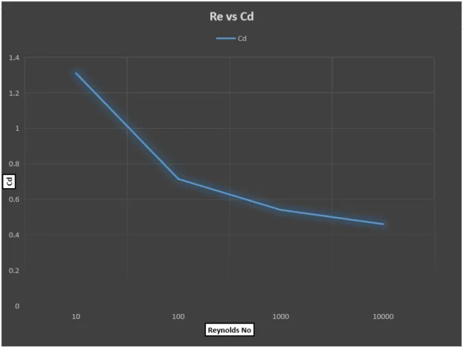
2. To calculate the coefficient of drag and lift over a cylinder by setting the Reynolds number to 10,100,1000,10000 & 100000. (Run with steady solver)
3. To discuss the effect of Reynolds number on the coefficient of drag.
4. To create a monitor point behind the cylinder at a distance 4 times the diameter which can be used to calculate and analyze the vortex shedding
5. Plots of the coefficient of drag and lift.
6. Plots to show vortex shedding behind the cylinder.

THEORY:

Karman Vortex street

The viscosity of the fluid makes the fluid to be attached with the Boundary layer of the cylinder in this case and to satisfy the no-slip condition the velocity will be zero. When the velocity decreases in the fluid flow there would no separation taking place in the boundary layer but when there is a high pressure gradient taking place the fluid particle have to over come the viscosity as well as the velocity increase which causes the fluid to move in opposite direction to the other leading to case called as the boundary layer separation. This boundary layer separation causes high turbulent region called as the wake. The pressure inside the wake remains low and as the flow separation occurs a net pressure force called drag is produced. Separating from the surface the boundary layer forms a shear layer which is unstable leading to the formation of Vortices. When the vortices from the top and bottom surface of the cylinder meet they form continuous vortices called as the Karman Vortex Street. This vortex shedding occurs at discrete frequency and its a function of Reynolds number. The Frequency of the Karman vortex is given by Strouhal Number Sr = f D/V, and is found to be approximately equal to 0.21 when Re > 1,000.

Here,

f is the frequency of the Vortices,

D is the diameter or the length in meters,

V is the velocity of the fluid in m/s.

Co-efficient of drag:

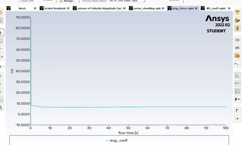
In fluid dynamics, the drag coefficient(Cd) is a dimensionless quantity that is used to quantify the drag or resistance of an object in a fluid environment, such as air or water. It is used in the drag equation in which a lower drag coefficient indicates the object will have a less aerodynamic or hydrodynamic drag. The drag coefficient is always associated with a particular surface area.

The drag coefficient of any object comprises the effects of the two basic contributors to fluid dynamic drag: skin friction and form drag. The drag coefficient of a lifting airfoil or hydrofoil also includes the effects of lift-induced drag. The drag coefficient of a complete structure such as an aircraft also includes the effects of interference drag.

`underset(d)(C)=(2*underset(d)(F))/(rhou^2A)`

where:

Fd">Fdis the drag force, which is by definition the force component in the direction of the flow velocity,

ρ">ρ is the mass density of the fluid,

u">uis the flow speed of the object relative to the fluid,

A">A is the reference area.

Co-efficient of lift:

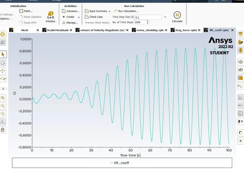
The lift coefficient CL is a dimensionless coefficient that relates the lift generated by a lifting body to the fluid density around the body, the fluid velocity, and an associated reference area. A lifting body is a foil or a complete foil-bearing body such as a fixed-wing aircraft. CL is a function of the angle of the body to the flow, its Reynolds number, and its Mach number. The section lift coefficient cl refers to the dynamic lift characteristics of a two-dimensional foil section, with the reference area replaced by the foil chord.

`underset(L)(C)=L/(qS)=L/(1/2*rhou^2S)=(2L)/(rhou^2S)`

where,

is the lift force,

is the relevant surface area .

PROCEDURE:

1:Pre Processing:

PROBLEM DEFNITION:

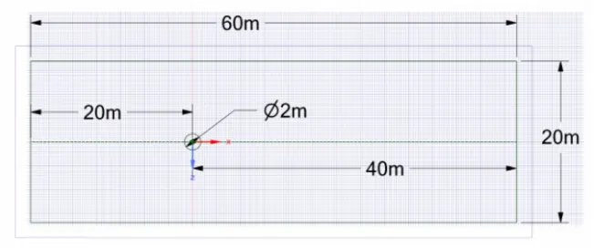
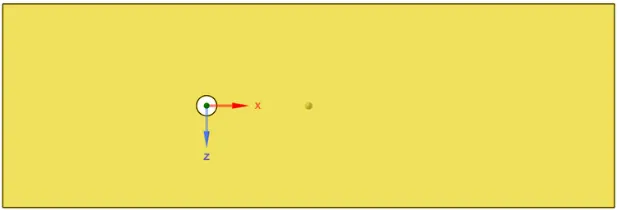
The problem is defined using SpaceClaim with a plate with the dimension of 20*60m and a cylinder with a diameter 0f 2m and the computational Domain of the problem is illustrated in the diagram below.

Geometry:

3d model:

2:MESH.

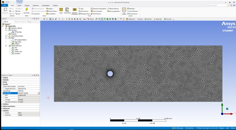
1. After the geometry is loaded we should mesh it. Mesh `rarr`Details of “Mesh”`rarr`Element Size In our case a mesh element size of 0.5m and mesh type as TRINANGLE is used, to insert mesh type Mesh `rarr`Insert`rarr`Methods`rarr`Geometry Select the geometry `rarr` Defnition `rarr` Method`rarr`Trinangles .
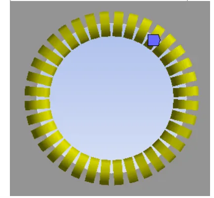
2. Then to capture the whole circumference of the cylinder, we can divide the circumference of the cylinder in 36 divisions, to define the divisions Mesh `rarr`Sizing`rarr`Details of sizing `rarr`Geometry select the edge of the cylinder`rarr` Defnition `rarr`Type `rarr`No of divisions .
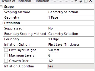
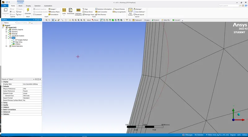
3. Then to insert Inflation `rarr` Geometry select the geometry`rarr` Boundary select the egde of the cylinder`rarr`Inflation `rarr` Option `rarr` First layer thicknes `rarr` First layer height define the required layer thickness, in our case we are using 5mm `rarr`Max layers define the required layers of inflation, here we are using 6 layers.
4. Then we have to assign names for the geometry.

Edge Sizing:

Inflation layer:

Final mesh with namings:

3:Solving:

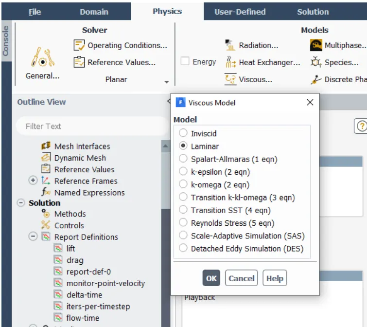
1. Workbench →Project schematic→ Setup → Physics`rarr` Laminar since we are doing only flow simulations.
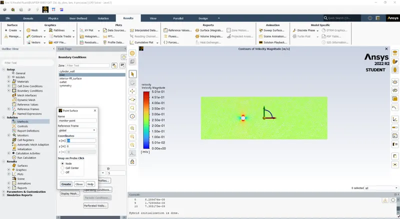
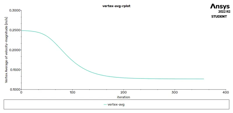
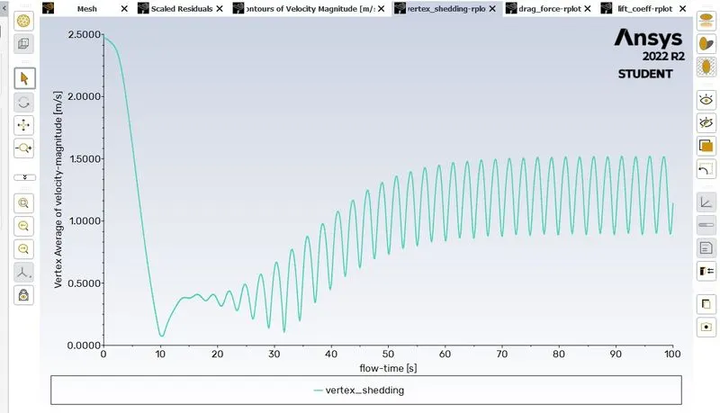
2. To get the velocity output we have to setup a monitor point at that point we can read the velocity readings, we have to setup the point at the distance of 4d(d=diameter of the cylinder).To setup monitor point Results `rarr` Create`rarr`Points `rarr` Name give the name as monitor point`rarr` the define the Location of the point.
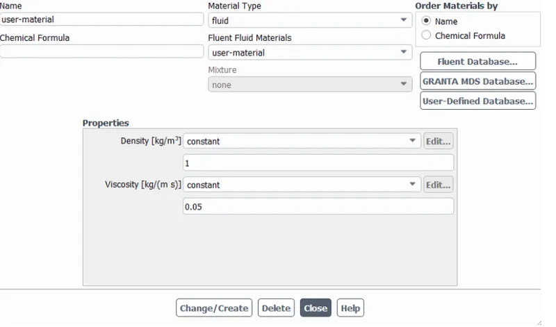
3. As we wanted to customize material property for simulation, go to Materials `rarr` fluent database `rarr` select the material (air)`rarr` copy it`rarr` rename the name of material change the fulid properties.

Viscous flow:

Monitor point:

Custamised material:

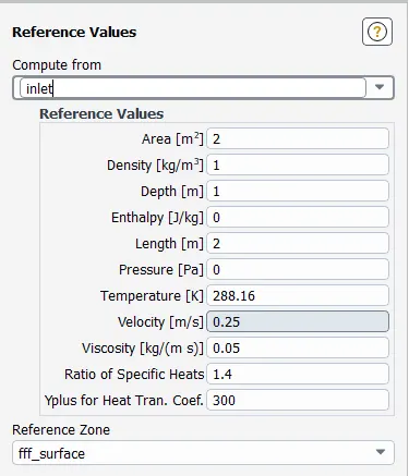
Reference value:

Velocity calculation:-

`V=(mu*underset(e)R)/(rho*D)` m/s

Re= Reynolds number,

Diameter, D= 2 m,

Density, `rho=1 (kg)/m^3`,

Dynamic Viscosity `mu=0.05( kg)/(ms)`,

Reynolds number	Velocity m/s
10	0.25
100	2.5
1000	25
10000	250
100000	2500

Steady state simulation:

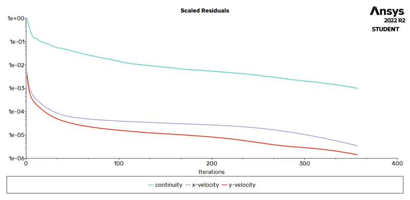
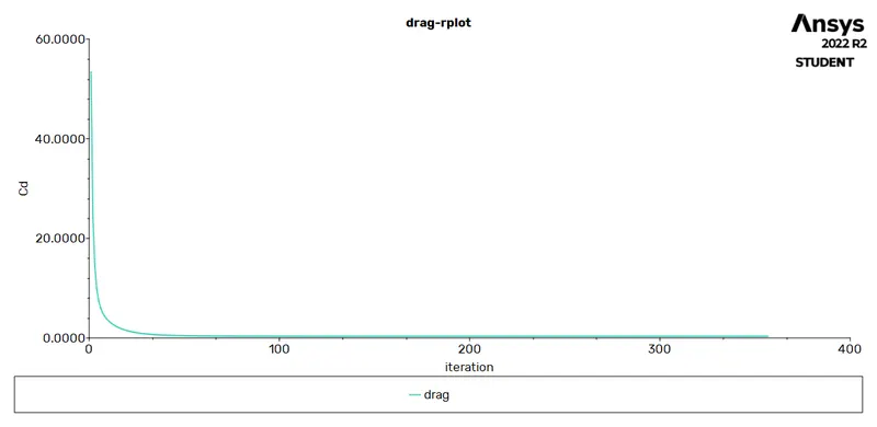
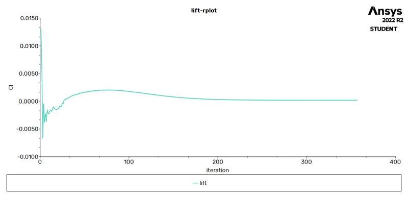
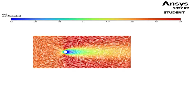
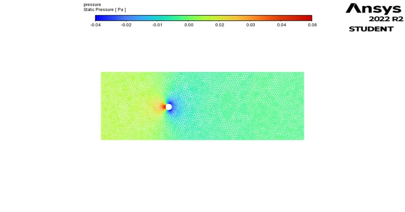
1.Reynolds number = 10.

velocity = 0.25 m/s.

density = 1 kg/m3.

viscosity = 0.05kg/ms.

`rarr`Residual plot:

`rarr`Velocity at monitor point:

`rarr`Drag:

`rarr`Lift:

`rarr` Velocity contour:

`rarr`Pressure contour:

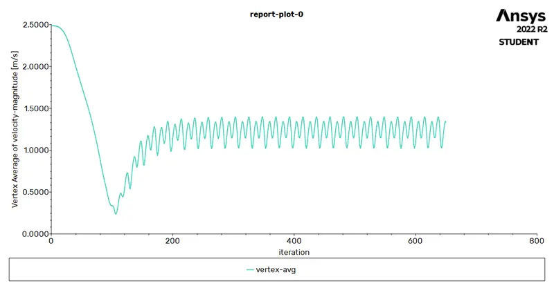
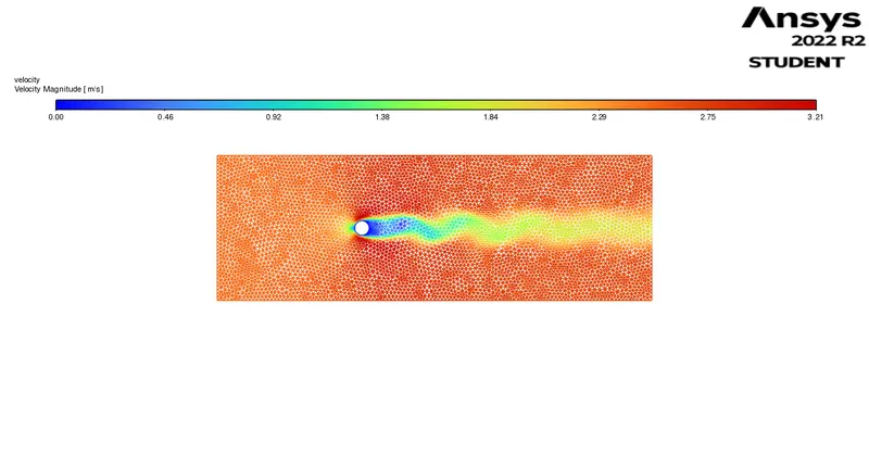
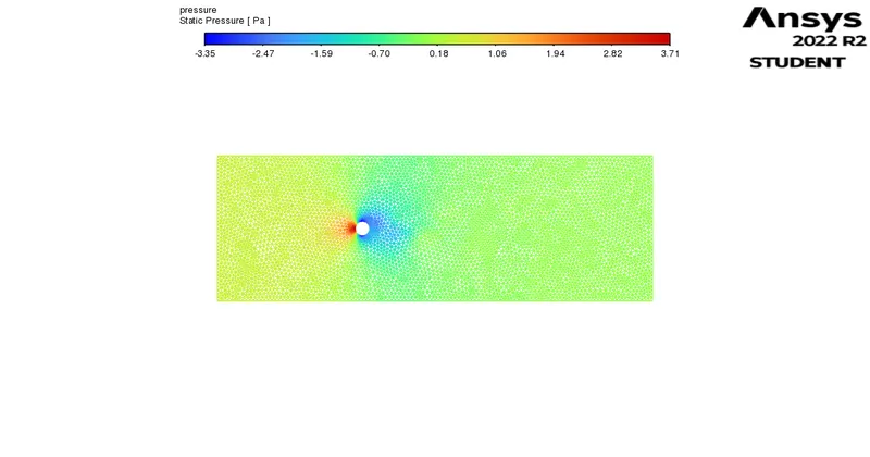
2.Reynolds number = 100.

velocity = 2.5 m/s.

density = 1 kg/m3.

viscosity = 0.05kg/ms.

`rarr`Scaled Residual:

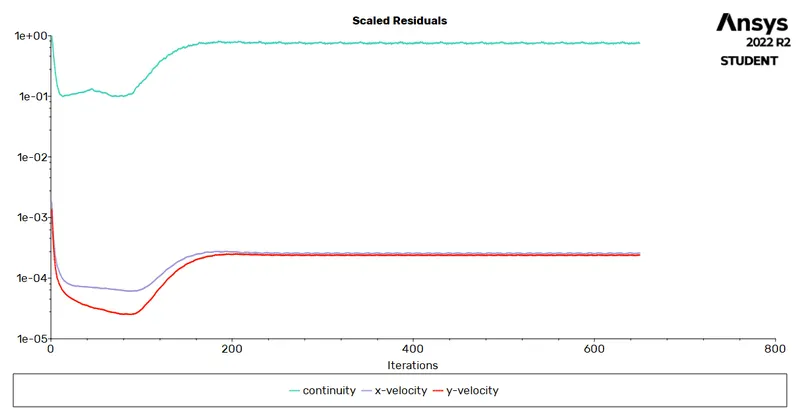
`rarr`Velocity at monitor point:

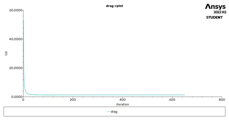
`rarr`Drag:

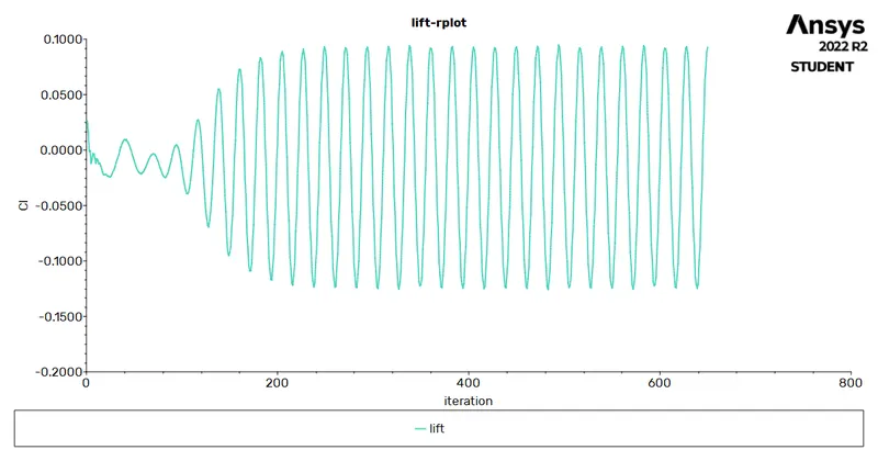
`rarr`Lift:

`rarr`Velocity contour:

`

`rarr`Pressure contour:

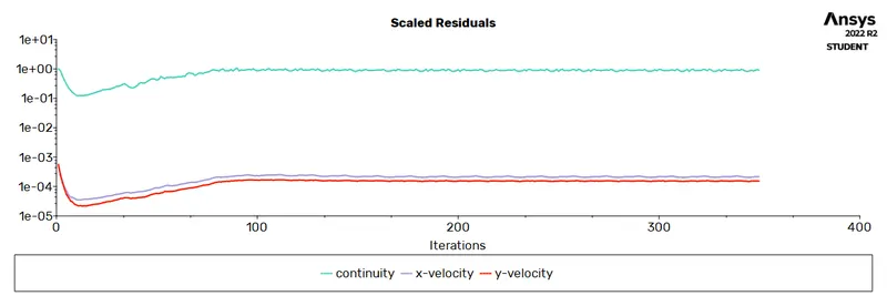
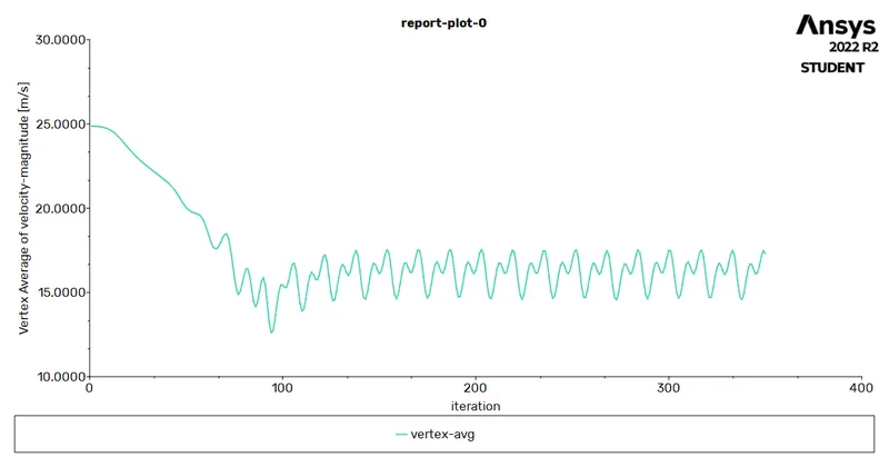
3.Reynolds number = 1000.

velocity = 25 m/s.

density = 1 kg/m3.

viscosity = 0.05kg/ms.

`rarr`Scaled Residual:

`rarr`Velocity at monitor point:

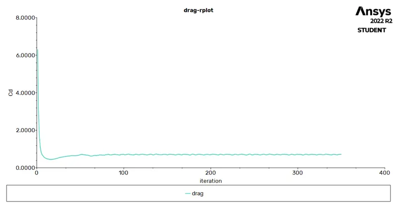
`rarr`Drag:

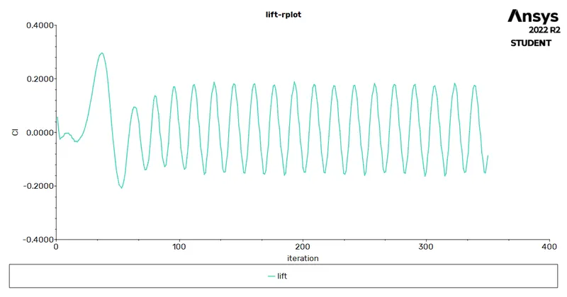
`rarr`Lift:

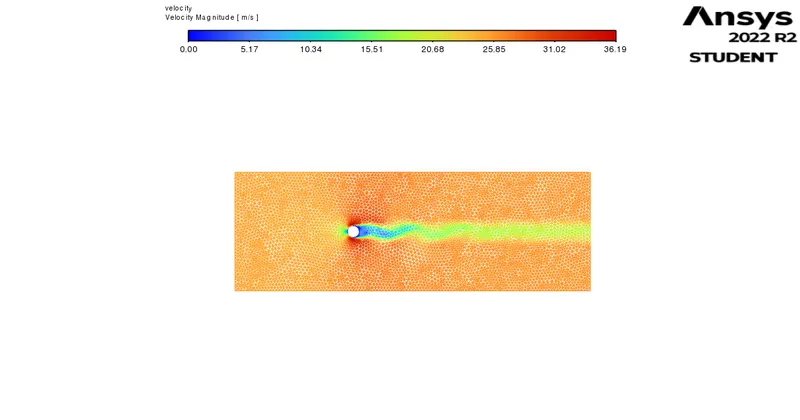
`rarr`Velocity contour:

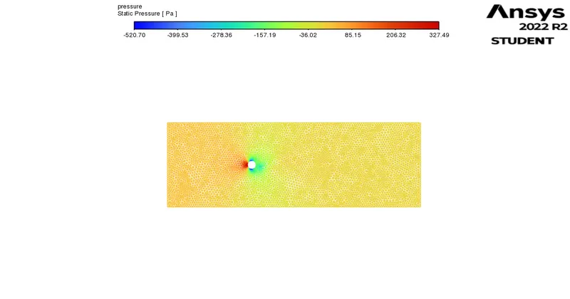
`rarr`Pressure contour:

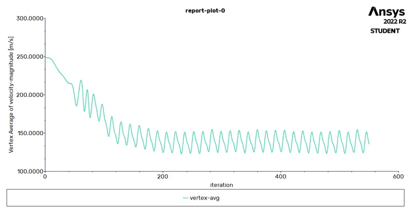
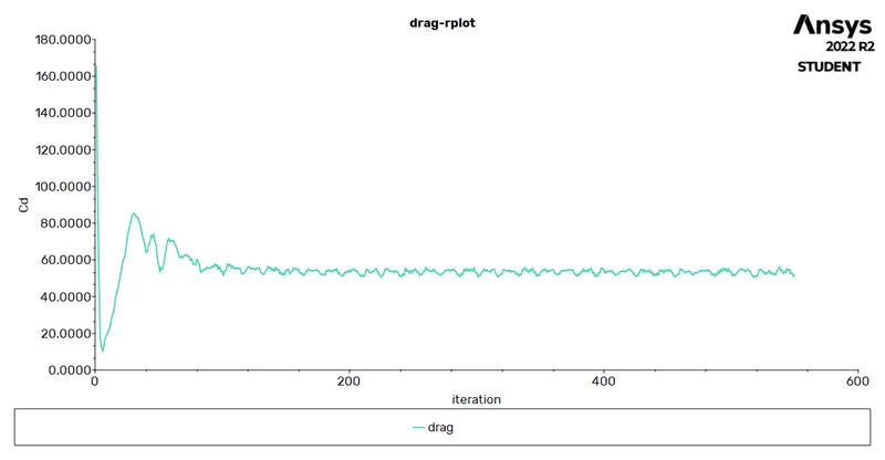
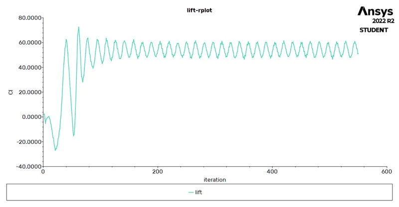
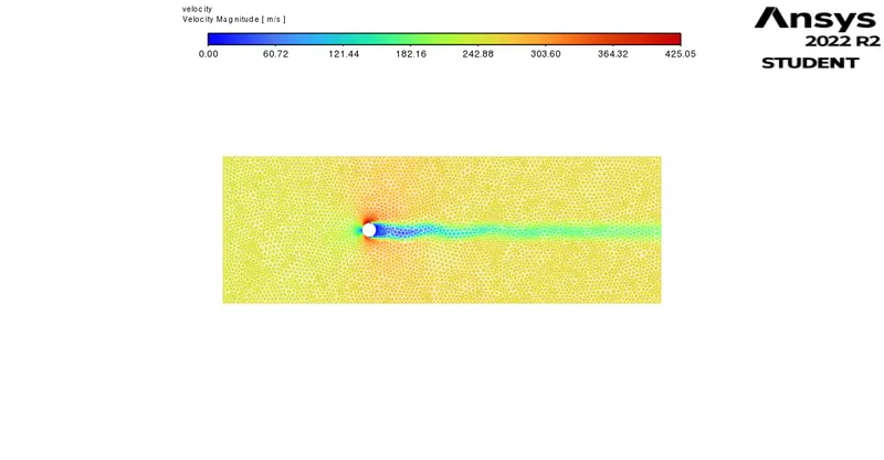
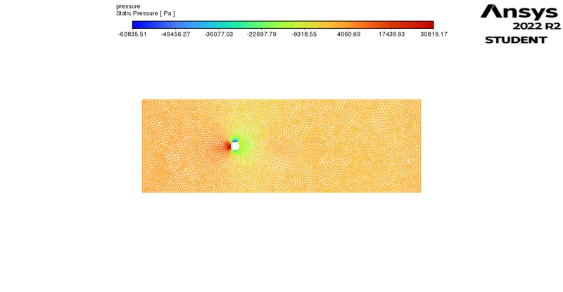
4.Reynolds number = 10000.

velocity = 250 m/s.

density = 1 kg/m3.

viscosity = 0.05kg/ms.

`rarr`Scaled Residual:

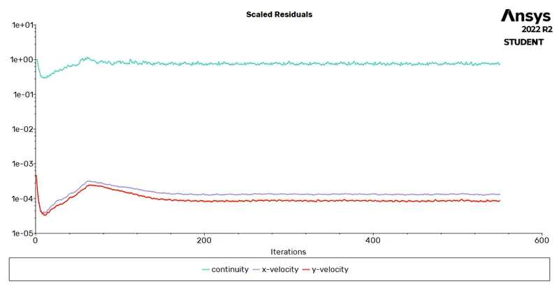
`rarr`Velocity at monitor point:

`rarr`Drag:

`rarr`Lift:

`rarr`Velocity contour:

`rarr`Pressure contour:

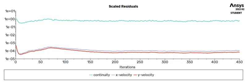
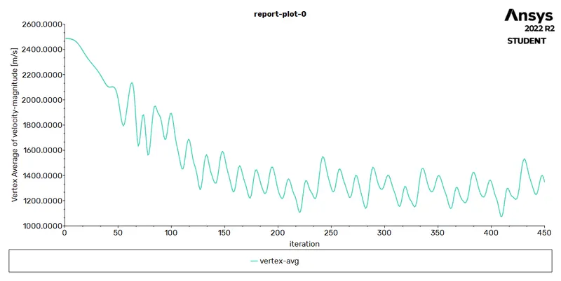
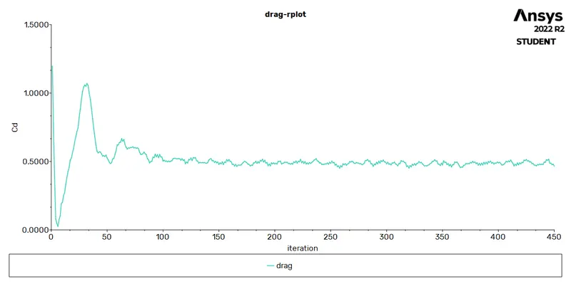
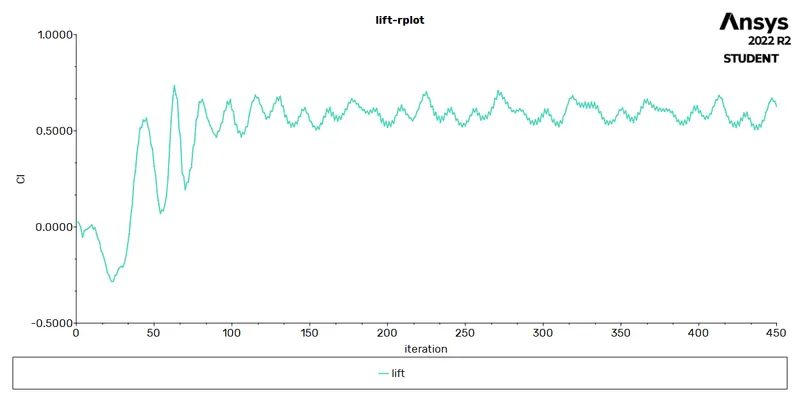
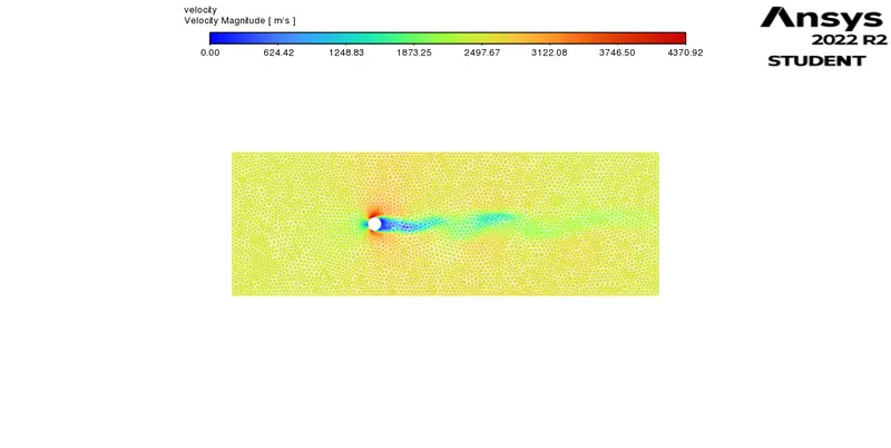
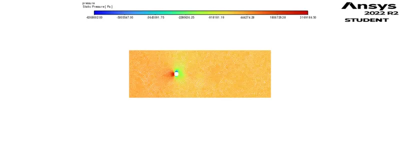
5.Reynolds number = 100000.

velocity = 2500m/s.

density = 1 kg/m3.

viscosity = 0.05kg/ms.

`rarr`Scaled Residual:

`rarr`Velocity at monitor point:

`rarr`Drag:

`rarr`Lift:

`rarr`Velocity contour:

`rarr`Pressure contour:

Unsteady state simulation:

Reynolds number = 100.

velocity = 2.5 m/s.

density = 1 kg/m3.

viscosity = 0.05kg/ms.

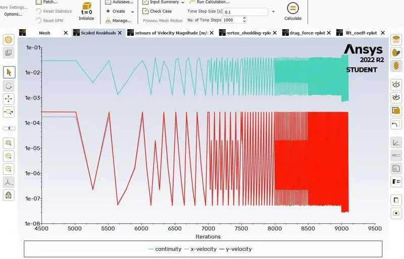
`rarr`Sacaled residual:

`rarr` Velocity at monitor point:

`rarr`Darg:

`rarr`Lift:

`rarr`Velocity contour:

`rarr`Pressure contour:

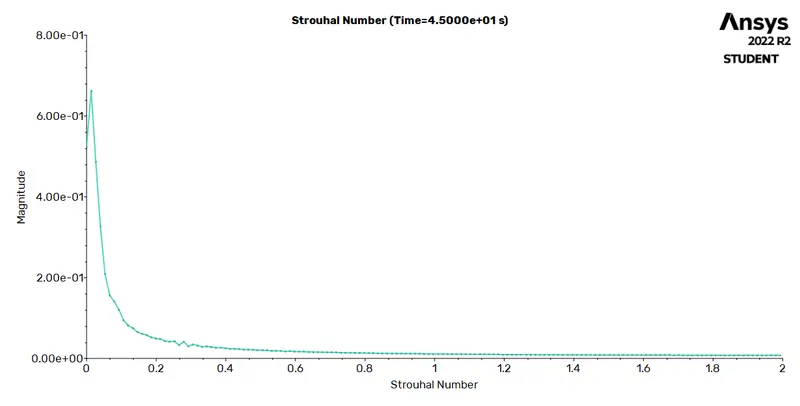
Strauhall number:

Strouhal number is a dimensionless number describing oscillating flow mechanisms.

The Strouhal number is often given as

St = f*d/u

Here,we have calculated staruhal no.using ansys fluent.

1.Go to fluent solver > results > fft analyser > load lift coefficient fiel > select plot FFT

Here, x axis denotes strauhal number and y axis denotes magnitude.

2.To get the magnitude of strauhal number,

go to results > fft analyser > click on write fft to file > click on write fft.

open the file in excel and 1st coloumn denotes the frequncy and 2nd coloumn denotes strauhal number.use the command max and select 2nd row and find the magnitude of strauhal number.

Reynold no vs Cd:

Conclusions:-

1. As the reynolds number increases Drag coefficient Decreases and lift coefficient increases.
2. Transient state capture more accurate vortex sheding than steady state solving.