Week 2 - Flow over a Cylinder.

Aim:

1. To simulate the flow over a cylinder and study the nature of steady and unsteady flows for a given Reynolds number.
2. Simulate flow over a cylinder and study the variation in the drag coefficient for various Reynolds numbers.

Objective:

To conduct flow simulation over a three-dimensional cylinder would require a very huge computational domain. The large size of the domain would also require proportionally large number of mesh elements. Hence, we would reduce the cylinder to a sphere in two dimensions and conduct a thorough investigation in the flow physics. We have two objectives:

1. To simulate the flow over a cylinder and study the nature of steady and unsteady flows for Re=100 and calculate Strouhal number.
2. Simulate flow over a cylinder in steady state and study the variation in the drag coefficient for five Reynold numbers- 10, 100, 1000, 10000, 100000.

Introduction:

Experiments performed to study the physics of certain phenomenon is costly and time-consuming. Numerical simulation is developed and used to reduce the time needed to study the nature and physics of the system of interest. This method indeed provides results very fast compared to experiments but they lack a bit in terms of accuracy. If the experiments take a month to produce results, simulation might take a day and give us results 90% accurate. In the fast-paced world, where developing various solutions require faster results, engineers make a delicate balance between the accuracy and time taken as necessary.

All fluid flows are governed by three equations -Continuity, momentum and energy equations. We need to solve these equations for the given conditions to understand the fluid behavior. Computers are incapable of solving these equations in their integral and differential forms. So, we can divide our geometry into many tiny elements (called mesh) and modify the governing equations into difference equations that can be solved by the computer. We apply these difference equations for all the elements in the geometry and generate an approximate solution. It is hence necessary to validate these results against the experimental data.

The number of difference equations, for a given problem varies with the nature of physics involved. We typically solve a finite number of equations at all the elements. These equations are grouped together, called a turbulence model. A lot of work has been put into developing and improving the turbulence models and the work still goes on today. Examples of turbulence models are S-A, k-epsilon, k-omega etc.

Theory:

Von-Karman vortex street:

When a fluid flows over a bluff body like a cylinder in this case, the fluid stream is cut by the body into two portions. Scientifically, we can see this as separation of the flow occurs around the body. These two streams reattach after some time and become a single stream again. This would create a small portion devoid of the fluid (or fluid at very low density) just adjacent to the body downstream. This is called wake region.

During continuous flow, this wake region causes the formation of a repetitive pattern downstream which seems to oscillate like a transverse wave. This phenomenon is called vortex shedding. The periodic occurrence of this phenomenon is Von-Karman vortex street.

The oscillation occurs at a definitive frequency for given flow conditions and can be represented by a non-dimensional parameter – Strouhal number (St).

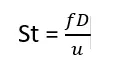
Where f = vortex shedding frequency (Hz)

D = diameter of the cylinder (m)

u = flow velocity (m/s).

Drag-coefficient:

When the fluid flows over the stationary body or vice-versa; the body offers a resistance to the fluid flow. This causes the fluid to exert force on the body which is termed drag-force. A non-dimensional parameter used to study this nature is called drag-coefficient (C_d).

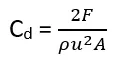
Where F = drag force (N)

ρ = density of the fluid (kg/m³)

u = flow velocity (m/s)

A = hydrodynamic area (m²)

Lift-coefficient:

When the fluid stream is split into two parts by the body, the pressure difference between the two streams causes a force to act through the body termed as Lift force. A non-dimensional parameter used to study this nature is called lift-coefficient (C_L).

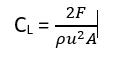
Where F = Lift force (N)

ρ = density of the fluid (kg/m³)

u = flow velocity (m/s)

A = hydrodynamic area (m²)

Modelling Approach:

The work flow in Ansys Fluent would follow four steps:

1. Geometry creation.
2. Mesh generation.
3. Pre-processing settings and simulation.
4. Extracting results.

Geometry creation:

We draw a circle of diameter D=2m, in the space claim. This would be our cylinder viewed in 2D. We would create a rectangular computational domain as shown in the following figure.

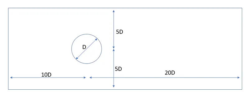
We create the surface in the drawn domain by using Pull option and delete the circle.

Mesh generation:

We will proceed with mesh generation for required mesh element length using the Sizing and Inflation options. We use Mesh -> Insert -> Sizing, to specify the number of the mesh elements in the given edge. We use Mesh -> Insert -> Inflation, to create inflation layers near the cylinder.

We assign appropriate named selections to make it easier to work in the simulation section later. Here, we assigned the flow inlets, outlet and wall. We close the window and the changes are updated in the system.

Pre-processing settings and Simulation:

We would proceed to Setup the conditions of the model. The process flow would be as follows:

1. Check the mesh in the solver.
2. Choose the turbulence model.
3. Specify boundary conditions.
4. Create necessary surface plots that we need to investigate.
5. We initialize and run the simulation for given number of iterations.
6. We set the reference values for area and length as 2m.

Extracting results:

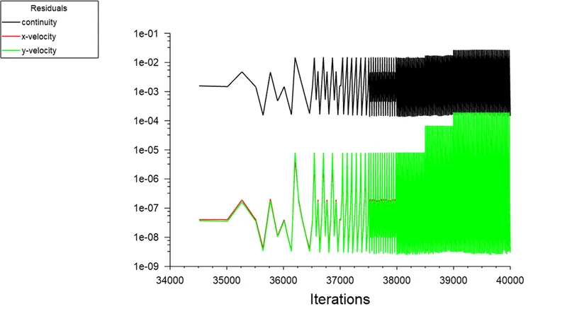
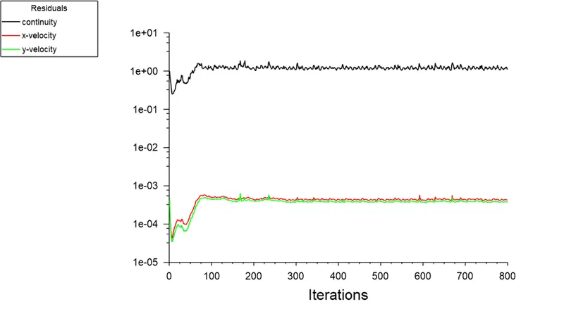
We open the results section where we can use various visualizing tools like transparency and colouring the created surfaces with the instantaneous variables like temperature, velocity and obtain contours and plots. We need to run the simulation until the residual values are either become constant or display a periodic pattern.

Settings used for current simulation:

We used Pressure-based solver, absolute velocity formulation, steady state simulation.

We used standard k-epsilon turbulence model. We define a new fluid as working fluid with specified properties.

Density of the fluid = 1 kg/m³

Dynamic viscosity = 0.05 Ns/m²

We can calculate the inlet velocity of the fluid for given Re as

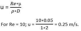
We have inlet velocities for other cases as:

Re	10	100	1000	1000	100000
U (m/s)	0.25	2.5	25	250	2500

Objective 1:

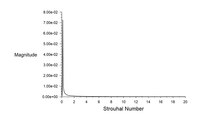
The first objective is to compare the results of steady and unsteady fluid flow for Re=100 and calculate the Strouhal number.

The only difference in pre-processor settings is that for steady flow we simulate the fluid flow for 800 iterations and for unsteady flow we simulate the flow for 40 seconds.

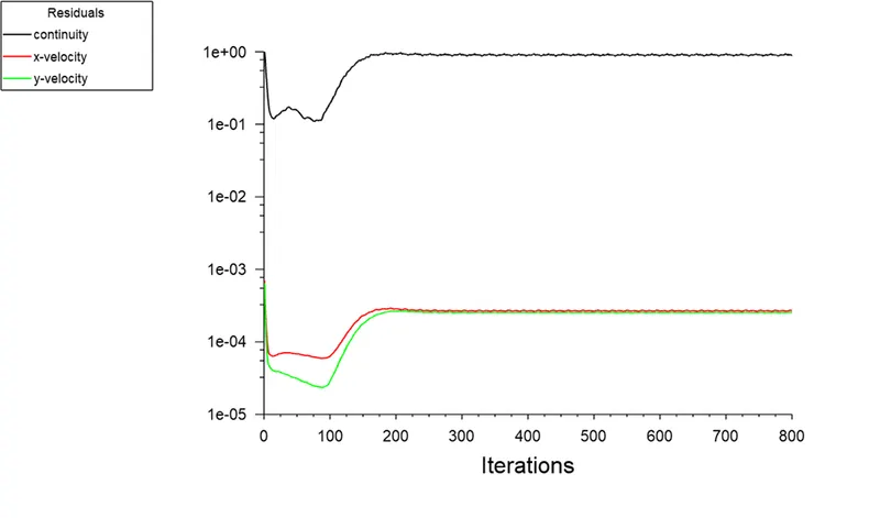
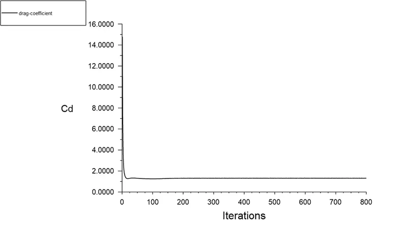
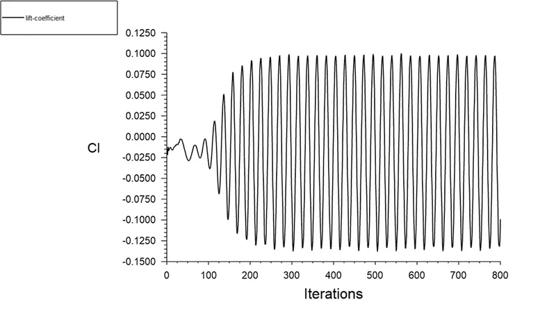
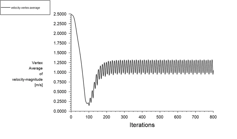
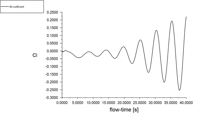
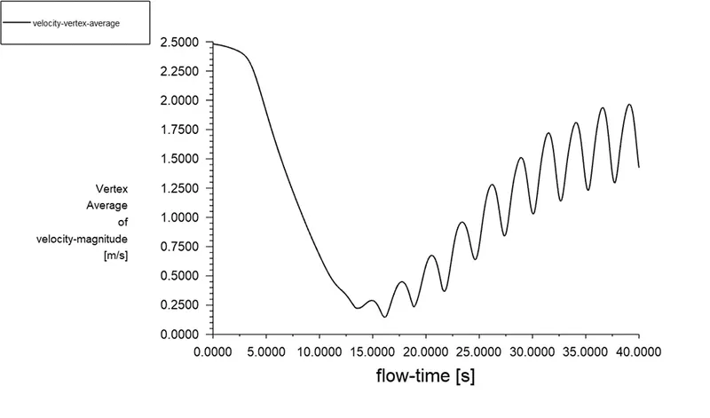
We have created a monitor point at a distance 4D from the surface of our cylinder. We get the following results:

Steady Flow:

Scaled residuals:

Drag coefficient:

Lift coefficient:

Velocity at vertex point:

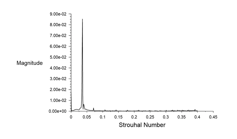
Strouhal number:

Unsteady Flow:

Scaled residuals:

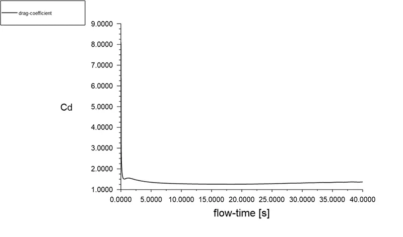
Drag coefficient:

Lift coefficient:

Velocity at vertex point:

Strouhal number:

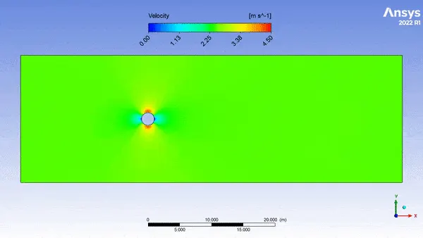
Animation:

Solver	Cd	CL	Maximum Strouhal no.
Steady	1.3152	-0.0991	0.0853
Unsteady	1.3691	0.2216	0.0727

Objective 2:

We would use steady solver to simulate the flow over the cylinder for five different Reynolds number.

The only parameter that changes for the following cases is the inlet velocity of the fluid. We input the velocity value as calculated earlier and observe the flow characteristics

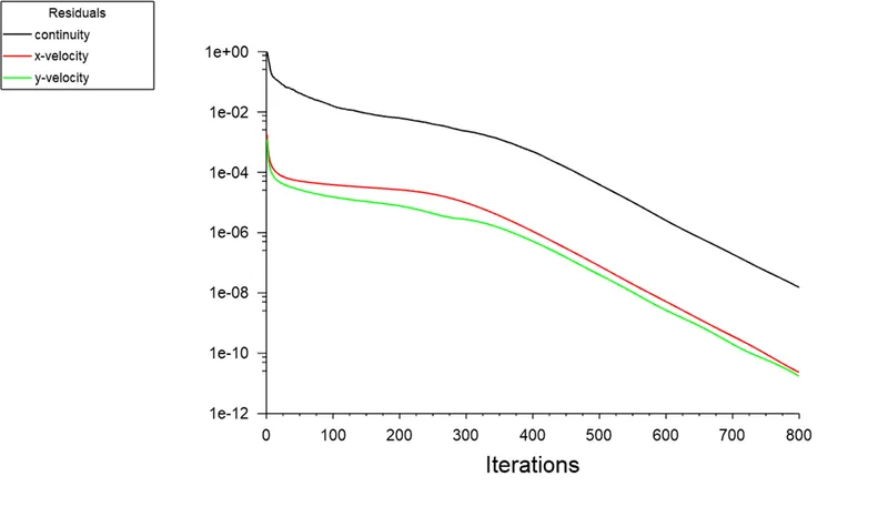
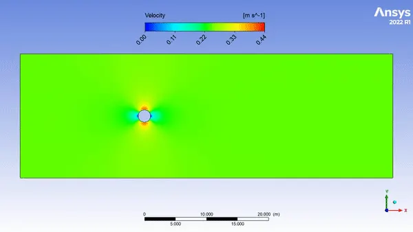
Case 1: Re = 10

Scaled residuals:

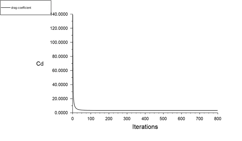
Drag coefficient:

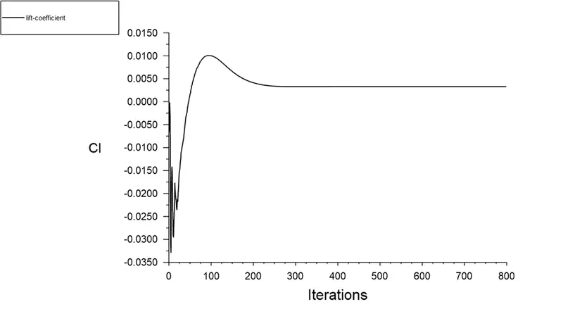
Lift coefficient:

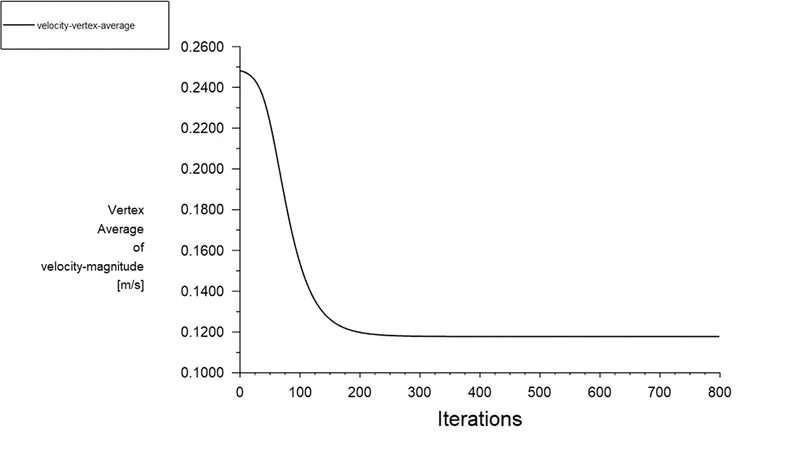
Velocity at vertex point:

Animation:

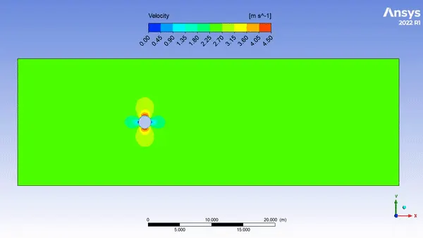
Case 2: Re = 100

Scaled residuals:

Drag coefficient:

Lift coefficient:

Velocity at vertex point:

Animation:

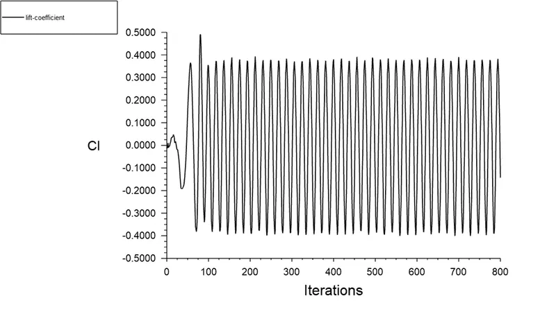
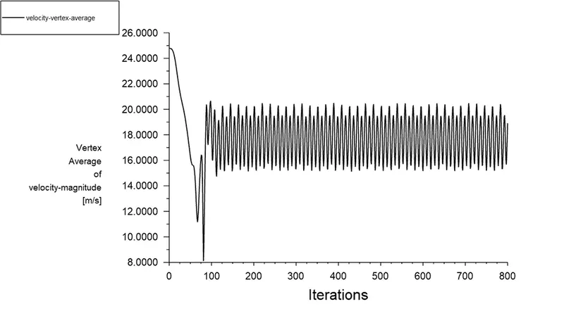
Case 3: Re = 1000

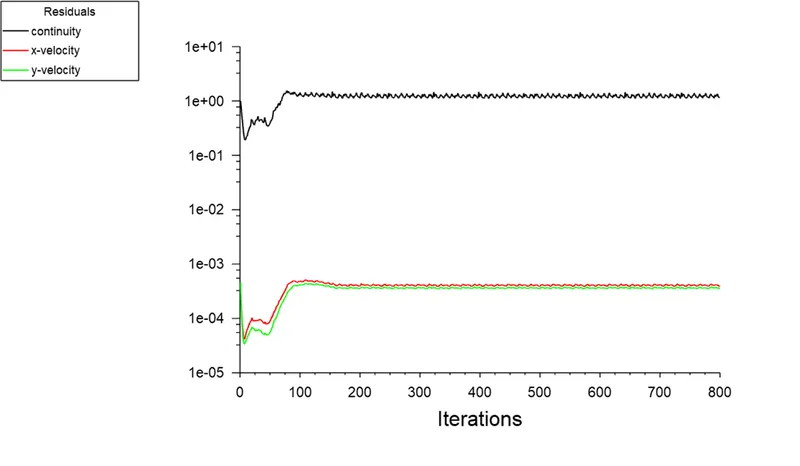
Scaled residuals:

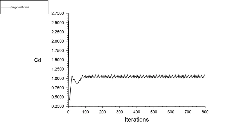
Drag coefficient:

Lift coefficient:

Velocity at vertex point:

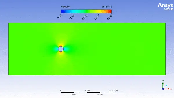
Animation:

Case 4: Re = 10000

Scaled residuals:

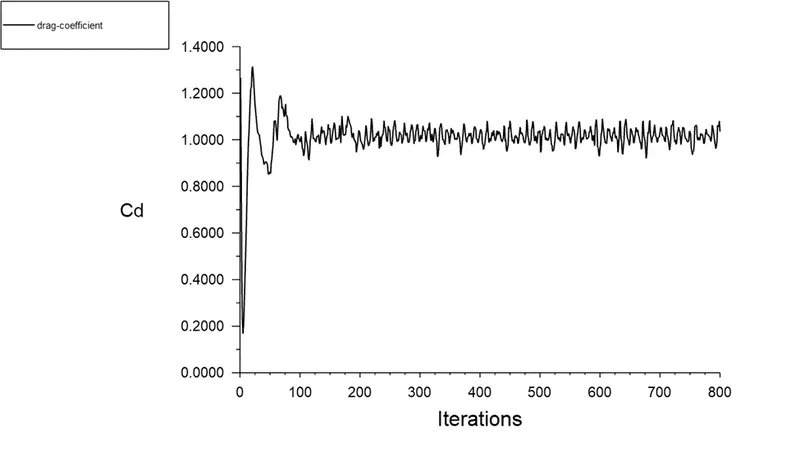
Drag coefficient:

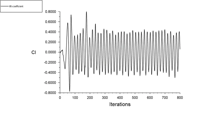
Lift coefficient:

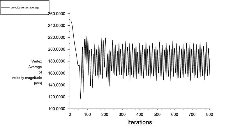
Velocity at vertex point:

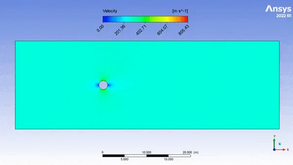
Animation:

Case 5: Re = 100000

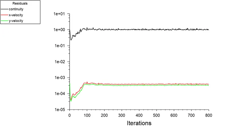
Scaled residuals:

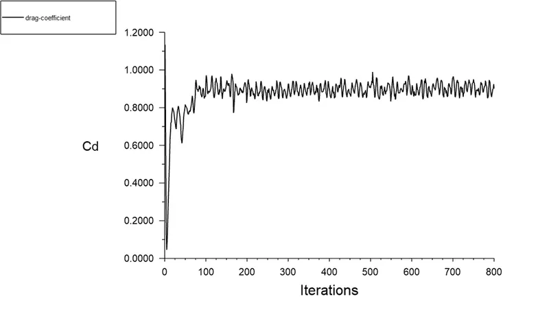
Drag coefficient:

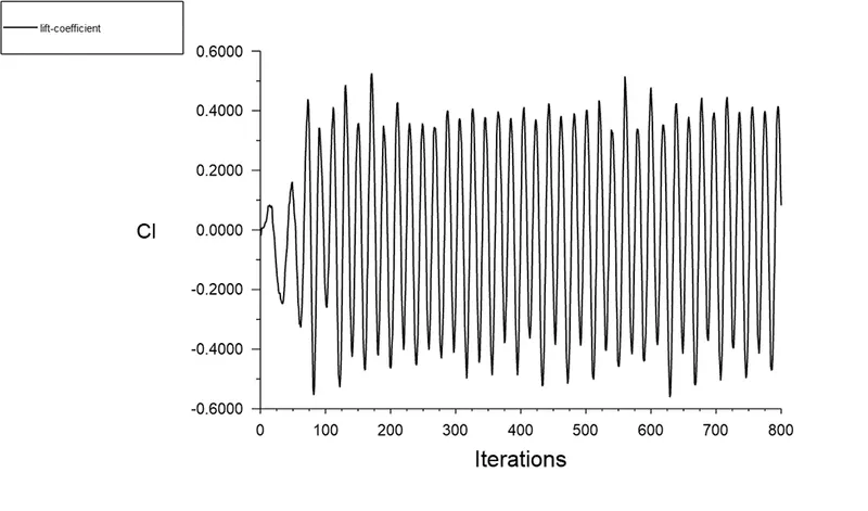
Lift coefficient:

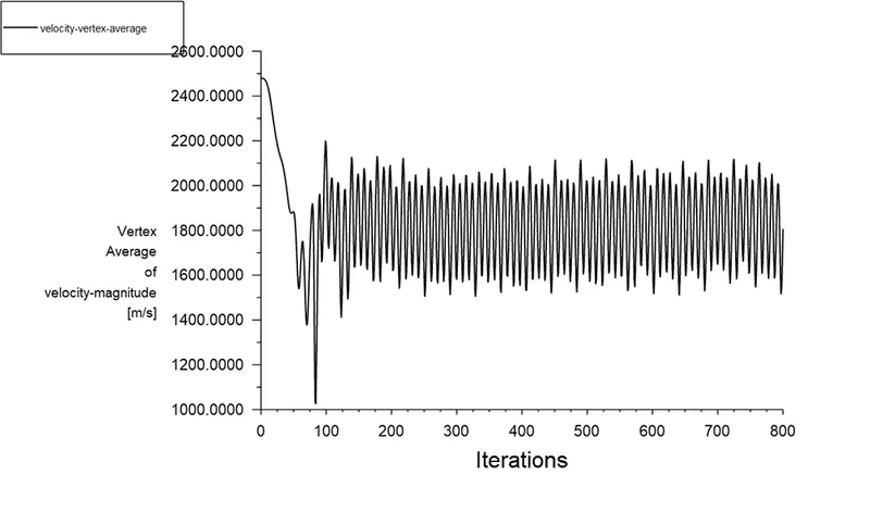
Velocity at vertex point:

Animation:

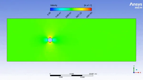
Results:

The average values of the drag and lift coefficients and velocity at the vertex are calculated and tabulated.

Re	Inlet velocity(m/s)	Cd	Velocity at vertex(m/s)
10	0.25	3.3086	0.12
100	2.5	1.3152	1.05
1000	25	1.031	18.91
10000	250	1.0353	184.47
100000	2500	0.9011	1806.74

Validation of results:

The simulation data should always be validated against the suitable experimental data in order to ensure that the chosen turbulence model gives the proper result. We can validate our results against the following graph obtained experimentally.

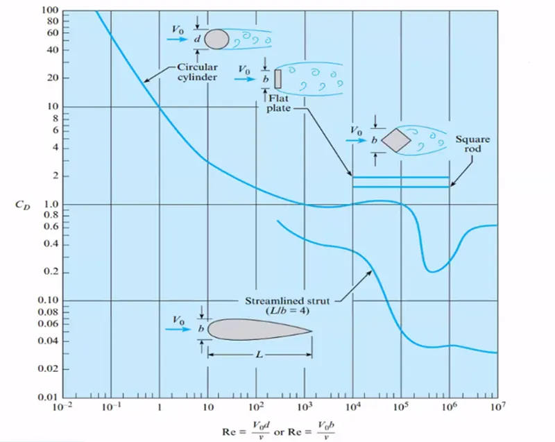
The data from the graph and the simulation are tabulated and deviation is calculated.

Re	Cd (experimental)	Cd (simulated)	Error (%)
10	3.33	3.308	2.2
100	1.34	1.315	2.5
1000	0.986	1.031	4.5
10000	1	1.0353	3.5
100000	0.954	0.9011	5.3

Conclusion:

The errors in the experimental and simulated values are very small. Hence, we can say the turbulence model captured the flow physics accurately.

References:

1. https://resources.system-analysis.cadence.com/blog/msa2022-correlation-of-the-drag-coefficient-vs-reynolds-number
2. Tudor Baracu, Grigoras-Benescu, Stefan, Computational Analysis of the flow around a cylinder and of the drag force, 2011.
3. N. Rajani, A. Kandasamy, Sekhar Majumdar, Numerical simulation of laminar flow past a circular cylinder, Applied Mathematical Modelling, Volume 33, Issue 3, 2009, Pages 1228-1247, ISSN 0307-904X
4. https://apps.automeris.io/wpd/ - Tool used to extract graphical data.