Week 2 - Flow over a Cylinder.
Aim : To simulate 2D flow over cylinder for varying Reynold number and observing the Coefficient of Drag, Lift, Strouhal no., Avg. vortex velocity for steady & transient flow. Further to study the von kormann vortex shedding phenomenon using Ansys Fluent.
Theory:
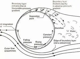
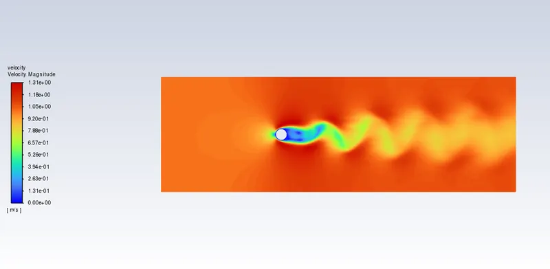
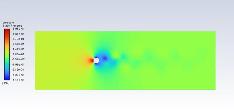
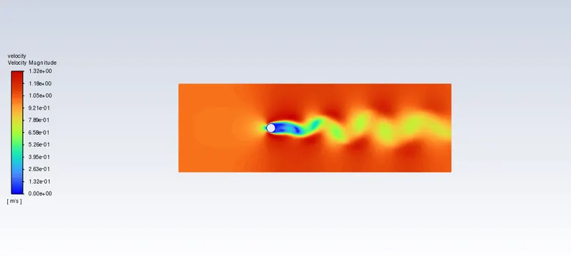
- When fluid flow over a cylinder wake generation starts to develop at the back of the cylinder. This wake generation starts to dominate when Reynolds Number is 100. This wake generation is named as Vortex shedding or von korman vortex shedding street.
- Due to this vortex shedding causes vibration on the structure. When this induced vibration matches with the natural resonance frequency, then it may lead to destruction.
- So in real life tall structures like chimney , buildings etc are constructed with varying diameter, fins to break the flow of fluid and prevent the wake generation.
- Due to this reason study of vortex shedding is really important
Ansys Simulation:
Geometry:
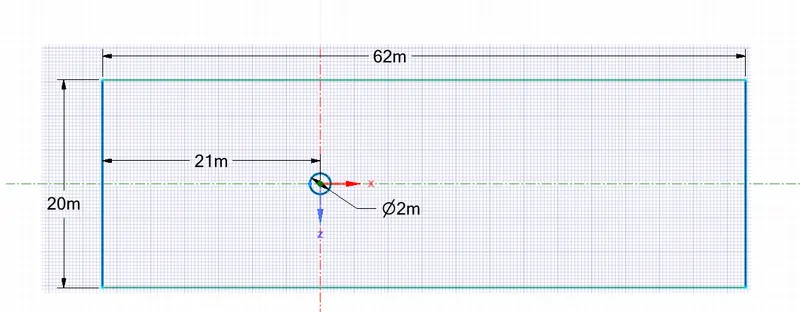
- The flow over the Cylinder is simulated by preparing the geometry in space claim.
- A circle is constructed at the origin of 2m diameter.
- The circle is enclosed within the rectangular boundary of 20m X 62m.
- The inlet boundary is 20m from the circle & outlet boundary be 40m from the circle.
- Top & Bottom boundary be symmetry boundary condition.
Mesh:
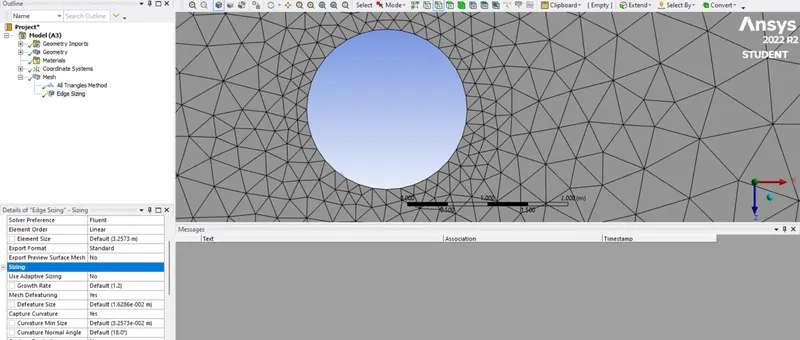
- The geometry is meshed by element size of .15m.
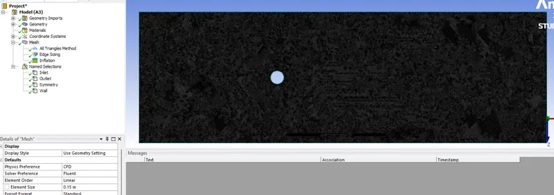
- Right click on Mesh and click on Method to Sizing, as the mesh near the circle is not uniform. In geometry select the edge of the circle and apply. Then select the no. of division to 36.
- Again, select Method Inflation mesh to Select first layer thickness and size of first layer to 0.005m.
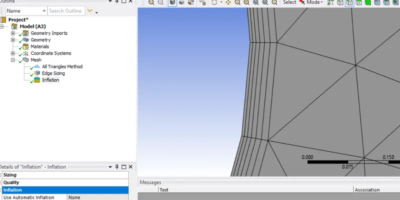
- The above method is performed to generate a body fitted mesh to capture vortex shedding through them.
Setup:
- Setup the simulation for steady state, laminar, Velocity absolute, Pressure based solver.
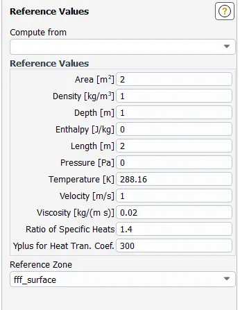
- Provide the reference values for the simulation Area to be projected area of cylinder, further as it is 2D simulation so Diameter of cylinder is taken at area. Then mention other parameters accordingly.
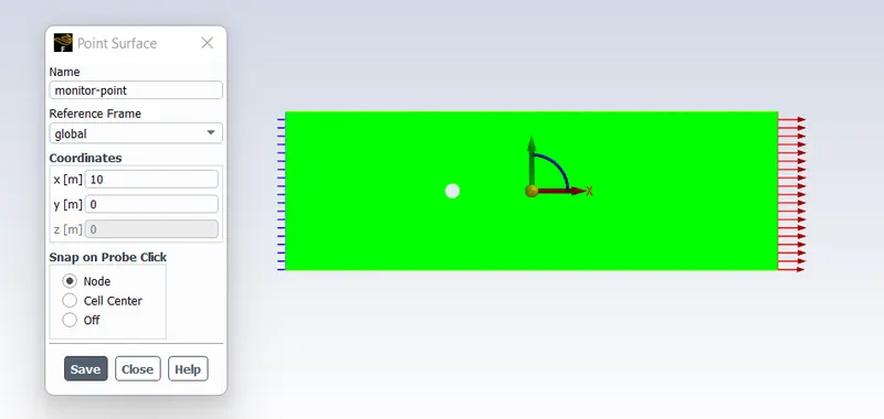
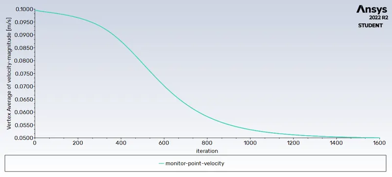
- Create monitoring point at a distance of 10m from the origin of circle and name it monitoring point.
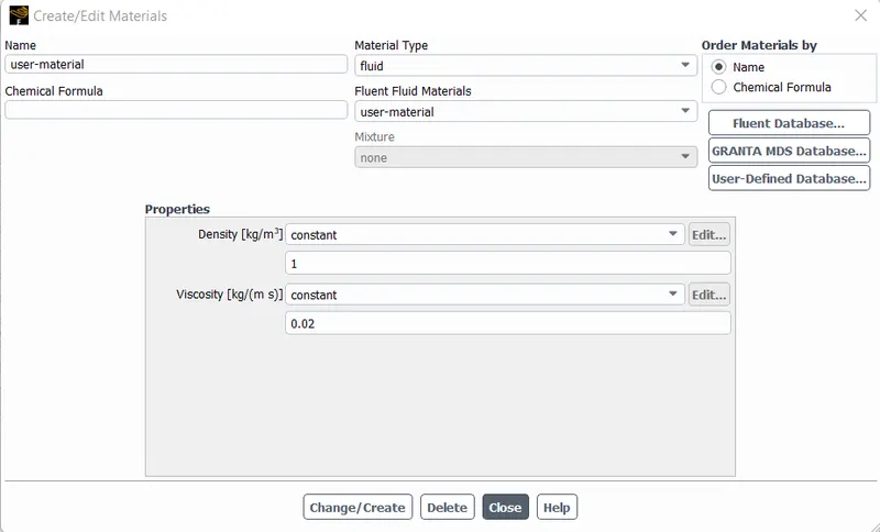
- In the Material section change the material properties to Density =1, Viscosity = 0.02. then press change.
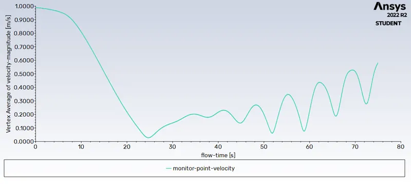
- Select definition surface report select vortex averaging select the monitoring point, similarly Generate coefficient of Drag & Lift plot as well.
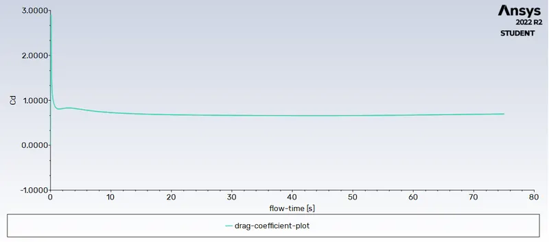
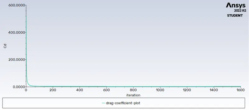
- Coefficient of Drag: It is a dimensionless quantity used to measure the drag on an object in a fluid environment.
`Cd=(Fd)/(0.5*rho*A*V^2`
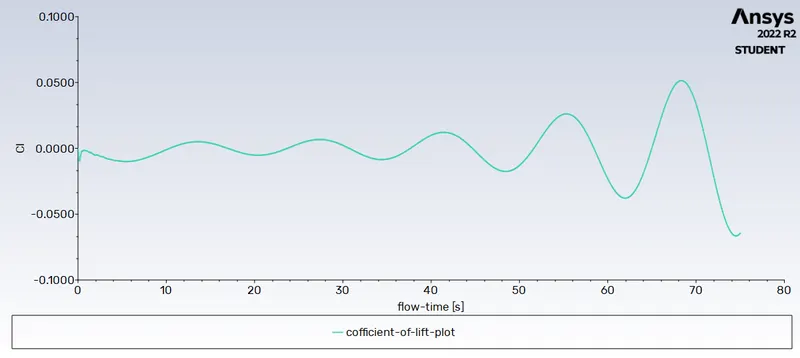
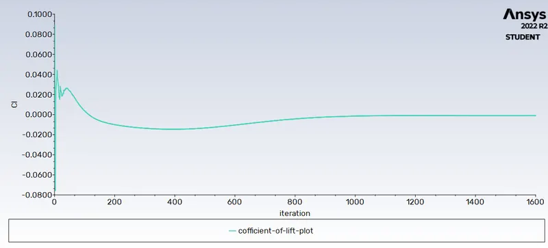
- Coefficient of Lift: It is a dimensionless quantity used to measure the Lift on an object in a fluid environment.
`Cl=(Fl)/(0.5*rho*A*V^2`
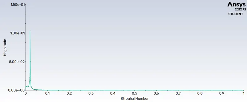
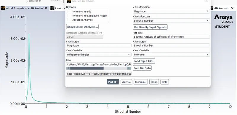
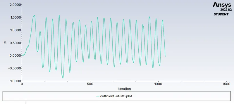
- In order to find the Strouhal Number we use the FFT plot i.e. fast Fourier transformation plot we take the input as lift plot and then in Y-axis magnitude and X-axis Strouhal number. Within the plot the highest magnitude corresponding is the required Strouhal number.
- Strouhal Number: It is dimensionless number which is used to describe the oscillating flow mechanisms.
`St=(f*L)/V`
Part A:
Simulate the flow over cylinder for steady and unsteady state for 100 Reynolds no. i.e. Inlet velocity is 1m/s, timestep = 0.1.
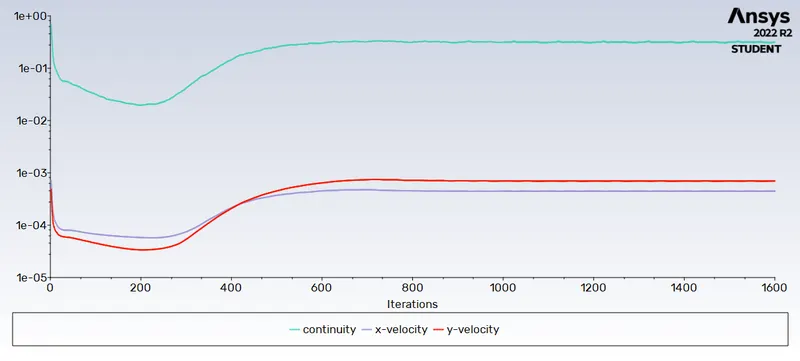
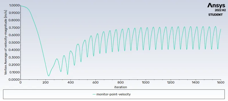
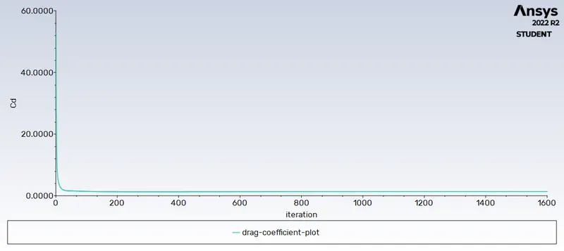
- Steady state flow for Reynolds no. is 100
Residual Plot:
Vortex Average Plot:
Coefficient of Drag Plot:
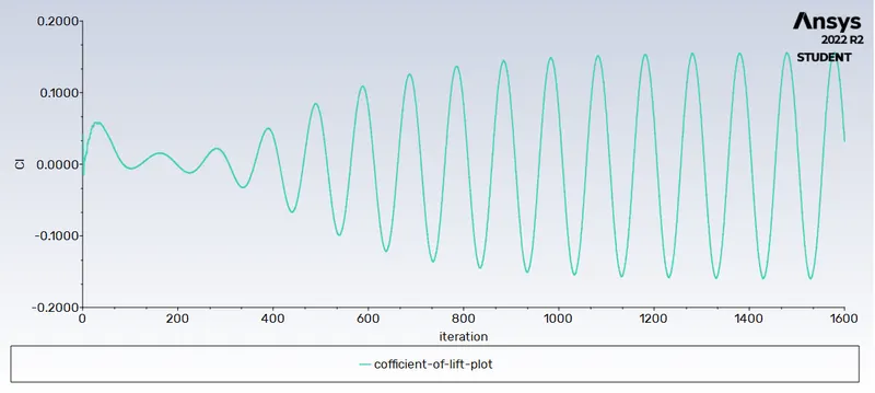
Coefficient of Lift Plot:
Strouhal Number Plot:
Velocity Contour:
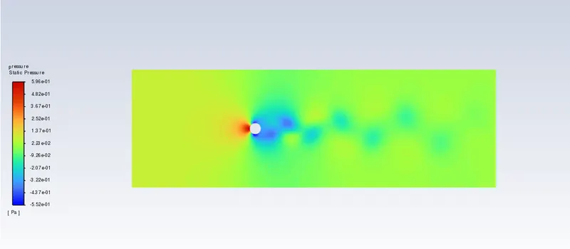
Pressure Contour:
- Transisent state flow for Reynolds no. is 100
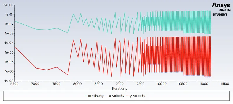
Residual Plot:
Vortex Average Plot:
Coefficient of Drag Plot:
Coefficient of Lift Plot:
Strouhal Number Plot:
Velocity Contour:
Pressure Contour:
Result_1:
| Sr.No. | Simulation | Coefficent of Drag | Coefficient of Lift | Strouhal Number |
| 1 | Steady | 1.3597 | 0.03234 | 0.021 |
| 2 | Transisent | 1.3247 | 0.05634 | 0.153 |
Part B:
Simulate the flow over cylinder for steady state of Reynolds no. 10, 1000, 10000, 100000
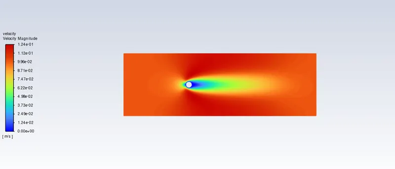
- Steady state flow for Reynolds No. 10, Inlet Velocity=0.1m/s.
Residual Plot:
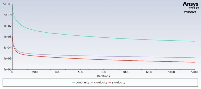
Vortex Average Plot:
Coefficient of Drag Plot:
Coefficient of Lift Plot:
Velocity Contour:
Pressure Contour:
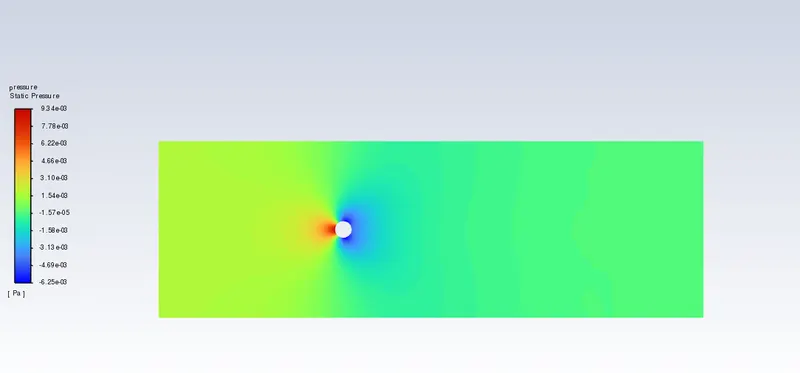
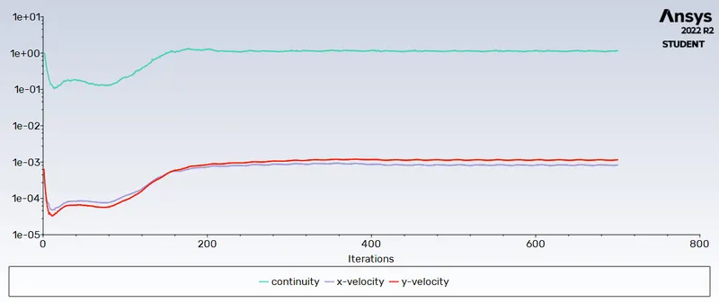
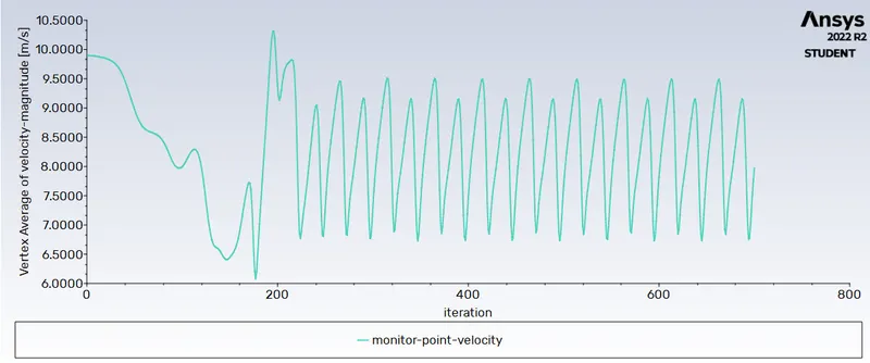
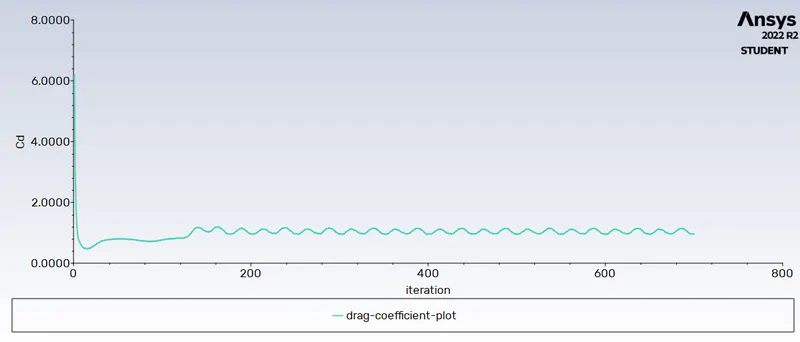
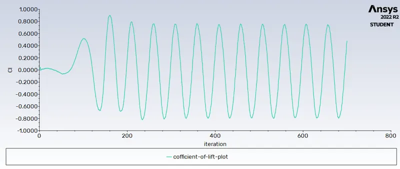
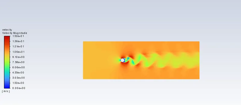
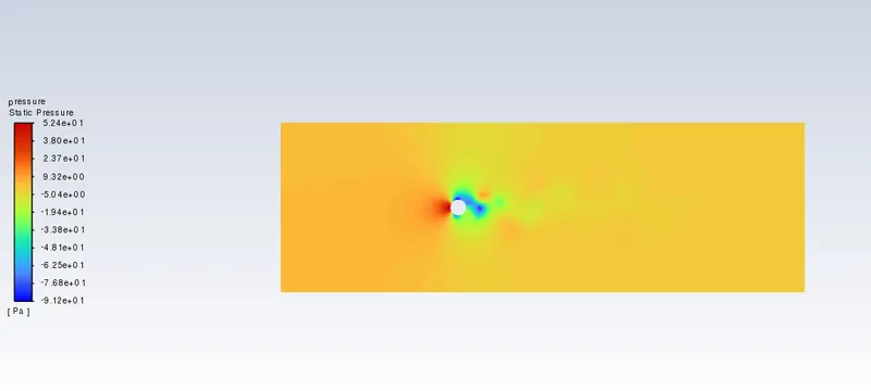
- Steady state flow for Reynolds No. 1000, Inlet Velocity=10m/s.
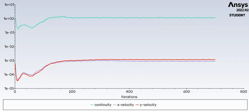
Residual Plot:
Vortex Average Plot:
Coefficient of Drag Plot:
Coefficient of Lift Plot:
Velocity Contour:
Pressure Contour:
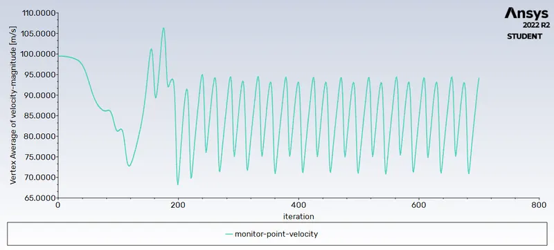
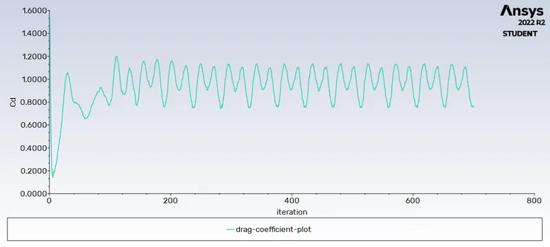
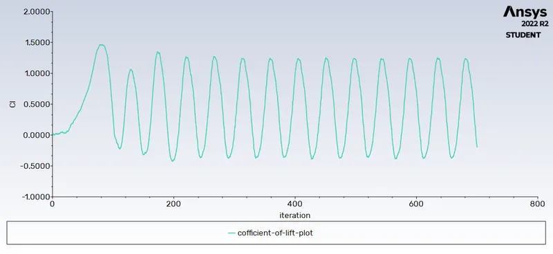
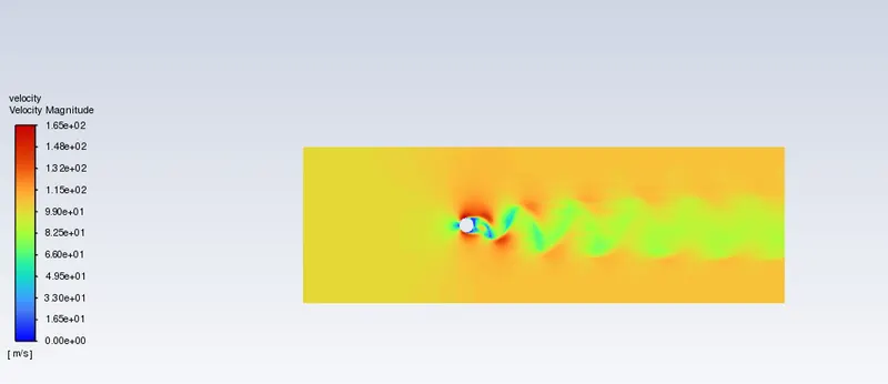
- Steady state flow for Reynolds No. 10000, Inlet Velocity=100m/s.
Residual Plot:
Vortex Average Plot:
Coefficient of Drag Plot:
Coefficient of Lift Plot:
Velocity Contour:
Pressure Contour:
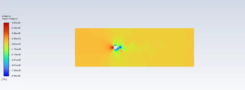
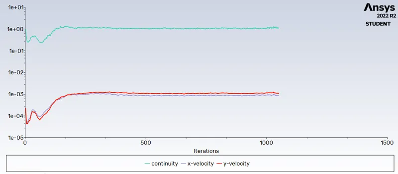
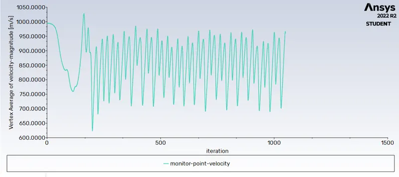
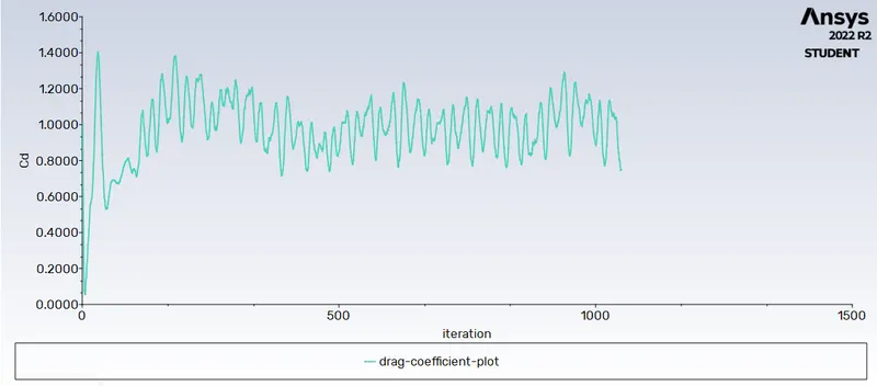
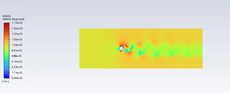
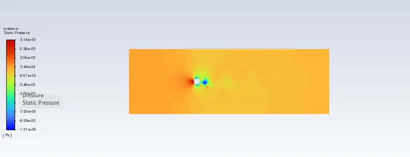
- Steady state flow for Reynolds No. 100000, Inlet Velocity=1000m/s.
Residual Plot:
Vortex Average Plot:
Coefficient of Drag Plot:
Coefficient of Lift Plot:
Velocity Contour:
Pressure Contour:
Result_2:
- After the Reynolds number 100 the vortex shedding can be observed.
- Inorder to get the result more accurate decrease the mesh element size and run the iteration for longer time, as the parameters are fluctuating hence as the no. of averageing terms incerease the result will lead near to actual.
Conclusion:
| Simulation | Reynolds Number | Cd (Numerical) | Cd (Therotical) | % Error | Ci (Numerical) |
| Staedy | 10 | 3.3331206 | 3.5 | 4.77 | -0.00105 |
| Steady | 100 | 1.3597108 | 1.4 | 2.88 | 0.032348 |
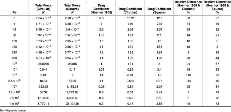
| Steady | 1000 | 1.1005178 | 1.31 | 15.99 | 0.525713 |
| Steady | 10000 | 0.7699081 | 0.89 | 13.49 | -0.19167 |
| Steady | 100000 | 0.74995166 | 0.64 | 17.17 | -0.045126 |
| Transient | 100 | 1.324709 | 1.4 | 5.377 | 0.0563425 |
- From the above table it is clear that as the reynolds number increase coefficient of drag decreases.
- The % errror for transisent state simulation is more as well as the simulation run time when comparing with similar reynolds number.
Reference:
A Numerical Analysis of Fluid Flow Around Circular and Square Cylinders - Scientific Figure on ResearchGate. Available from: https://www.researchgate.net/figure/Drag-force-and-drag-coefficient-at-different-Reynolds-numbers_tbl2_305876539 [accessed 19 Aug, 2022